T Test (Student’s T-Test): Definition and Examples
T Test: Contents :
- What is a T Test?
- The T Score
- T Values and P Values
- Calculating the T Test
- What is a Paired T Test (Paired Samples T Test)?

What is a T test?
The t test tells you how significant the differences between group means are. It lets you know if those differences in means could have happened by chance. The t test is usually used when data sets follow a normal distribution but you don’t know the population variance .
For example, you might flip a coin 1,000 times and find the number of heads follows a normal distribution for all trials. So you can calculate the sample variance from this data, but the population variance is unknown. Or, a drug company may want to test a new cancer drug to find out if it improves life expectancy. In an experiment, there’s always a control group (a group who are given a placebo, or “sugar pill”). So while the control group may show an average life expectancy of +5 years, the group taking the new drug might have a life expectancy of +6 years. It would seem that the drug might work. But it could be due to a fluke. To test this, researchers would use a Student’s t-test to find out if the results are repeatable for an entire population.
In addition, a t test uses a t-statistic and compares this to t-distribution values to determine if the results are statistically significant .
However, note that you can only uses a t test to compare two means. If you want to compare three or more means, use an ANOVA instead.
The T Score.
The t score is a ratio between the difference between two groups and the difference within the groups .
- Larger t scores = more difference between groups.
- Smaller t score = more similarity between groups.
A t score of 3 tells you that the groups are three times as different from each other as they are within each other. So when you run a t test, bigger t-values equal a greater probability that the results are repeatable.
T-Values and P-values
How big is “big enough”? Every t-value has a p-value to go with it. A p-value from a t test is the probability that the results from your sample data occurred by chance. P-values are from 0% to 100% and are usually written as a decimal (for example, a p value of 5% is 0.05). Low p-values indicate your data did not occur by chance . For example, a p-value of .01 means there is only a 1% probability that the results from an experiment happened by chance.
Calculating the Statistic / Test Types
There are three main types of t-test:
- An Independent Samples t-test compares the means for two groups.
- A Paired sample t-test compares means from the same group at different times (say, one year apart).
- A One sample t-test tests the mean of a single group against a known mean.
You can find the steps for an independent samples t test here . But you probably don’t want to calculate the test by hand (the math can get very messy. Use the following tools to calculate the t test:
- How to do a T test in Excel.
- T test in SPSS.
- T-distribution on the TI 89.
- T distribution on the TI 83.
What is a Paired T Test (Paired Samples T Test / Dependent Samples T Test)?
A paired t test (also called a correlated pairs t-test , a paired samples t test or dependent samples t test ) is where you run a t test on dependent samples. Dependent samples are essentially connected — they are tests on the same person or thing. For example:
- Knee MRI costs at two different hospitals,
- Two tests on the same person before and after training,
- Two blood pressure measurements on the same person using different equipment.
When to Choose a Paired T Test / Paired Samples T Test / Dependent Samples T Test
Choose the paired t-test if you have two measurements on the same item, person or thing. But you should also choose this test if you have two items that are being measured with a unique condition. For example, you might be measuring car safety performance in vehicle research and testing and subject the cars to a series of crash tests. Although the manufacturers are different, you might be subjecting them to the same conditions.
With a “regular” two sample t test , you’re comparing the means for two different samples . For example, you might test two different groups of customer service associates on a business-related test or testing students from two universities on their English skills. But if you take a random sample each group separately and they have different conditions, your samples are independent and you should run an independent samples t test (also called between-samples and unpaired-samples).
The null hypothesis for the independent samples t-test is μ 1 = μ 2 . So it assumes the means are equal. With the paired t test, the null hypothesis is that the pairwise difference between the two tests is equal (H 0 : µ d = 0).
Paired Samples T Test By hand

- The “ΣD” is the sum of X-Y from Step 2.
- ΣD 2 : Sum of the squared differences (from Step 4).
- (ΣD) 2 : Sum of the differences (from Step 2), squared.
If you’re unfamiliar with the Σ notation used in the t test, it basically means to “add everything up”. You may find this article useful: summation notation .

Step 6: Subtract 1 from the sample size to get the degrees of freedom. We have 11 items. So 11 – 1 = 10.
Step 7: Find the p-value in the t-table , using the degrees of freedom in Step 6. But if you don’t have a specified alpha level , use 0.05 (5%).
So for this example t test problem, with df = 10, the t-value is 2.228.
Step 8: In conclusion, compare your t-table value from Step 7 (2.228) to your calculated t-value (-2.74). The calculated t-value is greater than the table value at an alpha level of .05. In addition, note that the p-value is less than the alpha level: p <.05. So we can reject the null hypothesis that there is no difference between means.
However, note that you can ignore the minus sign when comparing the two t-values as ± indicates the direction; the p-value remains the same for both directions.
In addition, check out our YouTube channel for more stats help and tips!
Goulden, C. H. Methods of Statistical Analysis, 2nd ed. New York: Wiley, pp. 50-55, 1956.
- Search Search Please fill out this field.
What Is a T-Test?
Understanding the t-test, using a t-test, which t-test to use.
- T-Test FAQs
- Fundamental Analysis
T-Test: What It Is With Multiple Formulas and When To Use Them
Read how this calculation can be used for hypothesis testing in statistics
Adam Hayes, Ph.D., CFA, is a financial writer with 15+ years Wall Street experience as a derivatives trader. Besides his extensive derivative trading expertise, Adam is an expert in economics and behavioral finance. Adam received his master's in economics from The New School for Social Research and his Ph.D. from the University of Wisconsin-Madison in sociology. He is a CFA charterholder as well as holding FINRA Series 7, 55 & 63 licenses. He currently researches and teaches economic sociology and the social studies of finance at the Hebrew University in Jerusalem.
:max_bytes(150000):strip_icc():format(webp)/adam_hayes-5bfc262a46e0fb005118b414.jpg "what is t test in quantitative research")
A t-test is an inferential statistic used to determine if there is a significant difference between the means of two groups and how they are related. T-tests are used when the data sets follow a normal distribution and have unknown variances, like the data set recorded from flipping a coin 100 times.
The t-test is a test used for hypothesis testing in statistics and uses the t-statistic, the t-distribution values, and the degrees of freedom to determine statistical significance.
Key Takeaways
- A t-test is an inferential statistic used to determine if there is a statistically significant difference between the means of two variables.
- The t-test is a test used for hypothesis testing in statistics.
- Calculating a t-test requires three fundamental data values including the difference between the mean values from each data set, the standard deviation of each group, and the number of data values.
- T-tests can be dependent or independent.
Investopedia / Sabrina Jiang
A t-test compares the average values of two data sets and determines if they came from the same population. In the above examples, a sample of students from class A and a sample of students from class B would not likely have the same mean and standard deviation. Similarly, samples taken from the placebo-fed control group and those taken from the drug prescribed group should have a slightly different mean and standard deviation.
Mathematically, the t-test takes a sample from each of the two sets and establishes the problem statement. It assumes a null hypothesis that the two means are equal.
Using the formulas, values are calculated and compared against the standard values. The assumed null hypothesis is accepted or rejected accordingly. If the null hypothesis qualifies to be rejected, it indicates that data readings are strong and are probably not due to chance.
The t-test is just one of many tests used for this purpose. Statisticians use additional tests other than the t-test to examine more variables and larger sample sizes. For a large sample size, statisticians use a z-test . Other testing options include the chi-square test and the f-test.
Consider that a drug manufacturer tests a new medicine. Following standard procedure, the drug is given to one group of patients and a placebo to another group called the control group. The placebo is a substance with no therapeutic value and serves as a benchmark to measure how the other group, administered the actual drug, responds.
After the drug trial, the members of the placebo-fed control group reported an increase in average life expectancy of three years, while the members of the group who are prescribed the new drug reported an increase in average life expectancy of four years.
Initial observation indicates that the drug is working. However, it is also possible that the observation may be due to chance. A t-test can be used to determine if the results are correct and applicable to the entire population.
Four assumptions are made while using a t-test. The data collected must follow a continuous or ordinal scale, such as the scores for an IQ test, the data is collected from a randomly selected portion of the total population, the data will result in a normal distribution of a bell-shaped curve, and equal or homogenous variance exists when the standard variations are equal.
T-Test Formula
Calculating a t-test requires three fundamental data values. They include the difference between the mean values from each data set, or the mean difference, the standard deviation of each group, and the number of data values of each group.
This comparison helps to determine the effect of chance on the difference, and whether the difference is outside that chance range. The t-test questions whether the difference between the groups represents a true difference in the study or merely a random difference.
The t-test produces two values as its output: t-value and degrees of freedom . The t-value, or t-score, is a ratio of the difference between the mean of the two sample sets and the variation that exists within the sample sets.
The numerator value is the difference between the mean of the two sample sets. The denominator is the variation that exists within the sample sets and is a measurement of the dispersion or variability.
This calculated t-value is then compared against a value obtained from a critical value table called the T-distribution table. Higher values of the t-score indicate that a large difference exists between the two sample sets. The smaller the t-value, the more similarity exists between the two sample sets.
A large t-score, or t-value, indicates that the groups are different while a small t-score indicates that the groups are similar.
Degrees of freedom refer to the values in a study that has the freedom to vary and are essential for assessing the importance and the validity of the null hypothesis. Computation of these values usually depends upon the number of data records available in the sample set.
Paired Sample T-Test
The correlated t-test, or paired t-test, is a dependent type of test and is performed when the samples consist of matched pairs of similar units, or when there are cases of repeated measures. For example, there may be instances where the same patients are repeatedly tested before and after receiving a particular treatment. Each patient is being used as a control sample against themselves.
This method also applies to cases where the samples are related or have matching characteristics, like a comparative analysis involving children, parents, or siblings.
The formula for computing the t-value and degrees of freedom for a paired t-test is:
T = mean 1 − mean 2 s ( diff ) ( n ) where: mean 1 and mean 2 = The average values of each of the sample sets s ( diff ) = The standard deviation of the differences of the paired data values n = The sample size (the number of paired differences) n − 1 = The degrees of freedom \begin{aligned}&T=\frac{\textit{mean}1 - \textit{mean}2}{\frac{s(\text{diff})}{\sqrt{(n)}}}\\&\textbf{where:}\\&\textit{mean}1\text{ and }\textit{mean}2=\text{The average values of each of the sample sets}\\&s(\text{diff})=\text{The standard deviation of the differences of the paired data values}\\&n=\text{The sample size (the number of paired differences)}\\&n-1=\text{The degrees of freedom}\end{aligned} T = ( n ) s ( diff ) mean 1 − mean 2 where: mean 1 and mean 2 = The average values of each of the sample sets s ( diff ) = The standard deviation of the differences of the paired data values n = The sample size (the number of paired differences) n − 1 = The degrees of freedom
Equal Variance or Pooled T-Test
The equal variance t-test is an independent t-test and is used when the number of samples in each group is the same, or the variance of the two data sets is similar.
The formula used for calculating t-value and degrees of freedom for equal variance t-test is:
T-value = mean 1 − mean 2 ( n 1 − 1 ) × var 1 2 + ( n 2 − 1 ) × var 2 2 n 1 + n 2 − 2 × 1 n 1 + 1 n 2 where: mean 1 and mean 2 = Average values of each of the sample sets var 1 and var 2 = Variance of each of the sample sets n 1 and n 2 = Number of records in each sample set \begin{aligned}&\text{T-value}=\frac{\textit{mean}1-\textit{mean}2}{\sqrt{\frac{(n1-1)\times\textit{var}1^2+(n2-1)\times\textit{var}2^2}{n1+n2-2}\times\frac{1}{n1}+\frac{1}{n2}}}\\&\textbf{where:}\\&\textit{mean}1 \text{ and } \textit{mean}2=\text{Average values of each}\\&\text{of the sample sets}\\&\textit{var}1\text{ and }\textit{var}2=\text{Variance of each of the sample sets}\\&n1\text{ and }n2=\text{Number of records in each sample set}\end{aligned} T-value = n 1 + n 2 − 2 ( n 1 − 1 ) × var 1 2 + ( n 2 − 1 ) × var 2 2 × n 1 1 + n 2 1 mean 1 − mean 2 where: mean 1 and mean 2 = Average values of each of the sample sets var 1 and var 2 = Variance of each of the sample sets n 1 and n 2 = Number of records in each sample set
Degrees of Freedom = n 1 + n 2 − 2 where: n 1 and n 2 = Number of records in each sample set \begin{aligned} &\text{Degrees of Freedom} = n1 + n2 - 2 \\ &\textbf{where:}\\ &n1 \text{ and } n2 = \text{Number of records in each sample set} \\ \end{aligned} Degrees of Freedom = n 1 + n 2 − 2 where: n 1 and n 2 = Number of records in each sample set
Unequal Variance T-Test
The unequal variance t-test is an independent t-test and is used when the number of samples in each group is different, and the variance of the two data sets is also different. This test is also called Welch's t-test.
The formula used for calculating t-value and degrees of freedom for an unequal variance t-test is:
T-value = m e a n 1 − m e a n 2 ( v a r 1 n 1 + v a r 2 n 2 ) where: m e a n 1 and m e a n 2 = Average values of each of the sample sets v a r 1 and v a r 2 = Variance of each of the sample sets n 1 and n 2 = Number of records in each sample set \begin{aligned}&\text{T-value}=\frac{mean1-mean2}{\sqrt{\bigg(\frac{var1}{n1}{+\frac{var2}{n2}\bigg)}}}\\&\textbf{where:}\\&mean1 \text{ and } mean2 = \text{Average values of each} \\&\text{of the sample sets} \\&var1 \text{ and } var2 = \text{Variance of each of the sample sets} \\&n1 \text{ and } n2 = \text{Number of records in each sample set} \end{aligned} T-value = ( n 1 v a r 1 + n 2 v a r 2 ) m e an 1 − m e an 2 where: m e an 1 and m e an 2 = Average values of each of the sample sets v a r 1 and v a r 2 = Variance of each of the sample sets n 1 and n 2 = Number of records in each sample set
Degrees of Freedom = ( v a r 1 2 n 1 + v a r 2 2 n 2 ) 2 ( v a r 1 2 n 1 ) 2 n 1 − 1 + ( v a r 2 2 n 2 ) 2 n 2 − 1 where: v a r 1 and v a r 2 = Variance of each of the sample sets n 1 and n 2 = Number of records in each sample set \begin{aligned} &\text{Degrees of Freedom} = \frac{ \left ( \frac{ var1^2 }{ n1 } + \frac{ var2^2 }{ n2 } \right )^2 }{ \frac{ \left ( \frac{ var1^2 }{ n1 } \right )^2 }{ n1 - 1 } + \frac{ \left ( \frac{ var2^2 }{ n2 } \right )^2 }{ n2 - 1}} \\ &\textbf{where:}\\ &var1 \text{ and } var2 = \text{Variance of each of the sample sets} \\ &n1 \text{ and } n2 = \text{Number of records in each sample set} \\ \end{aligned} Degrees of Freedom = n 1 − 1 ( n 1 v a r 1 2 ) 2 + n 2 − 1 ( n 2 v a r 2 2 ) 2 ( n 1 v a r 1 2 + n 2 v a r 2 2 ) 2 where: v a r 1 and v a r 2 = Variance of each of the sample sets n 1 and n 2 = Number of records in each sample set
The following flowchart can be used to determine which t-test to use based on the characteristics of the sample sets. The key items to consider include the similarity of the sample records, the number of data records in each sample set, and the variance of each sample set.
Image by Julie Bang © Investopedia 2019
Example of an Unequal Variance T-Test
Assume that the diagonal measurement of paintings received in an art gallery is taken. One group of samples includes 10 paintings, while the other includes 20 paintings. The data sets, with the corresponding mean and variance values, are as follows:
| Set 1 | Set 2 | |
|---|---|---|
| 19.7 | 28.3 | |
| 20.4 | 26.7 | |
| 19.6 | 20.1 | |
| 17.8 | 23.3 | |
| 18.5 | 25.2 | |
| 18.9 | 22.1 | |
| 18.3 | 17.7 | |
| 18.9 | 27.6 | |
| 19.5 | 20.6 | |
| 21.95 | 13.7 | |
| 23.2 | ||
| 17.5 | ||
| 20.6 | ||
| 18 | ||
| 23.9 | ||
| 21.6 | ||
| 24.3 | ||
| 20.4 | ||
| 23.9 | ||
| 13.3 | ||
| 19.4 | 21.6 | |
| 1.4 | 17.1 |
Though the mean of Set 2 is higher than that of Set 1, we cannot conclude that the population corresponding to Set 2 has a higher mean than the population corresponding to Set 1.
Is the difference from 19.4 to 21.6 due to chance alone, or do differences exist in the overall populations of all the paintings received in the art gallery? We establish the problem by assuming the null hypothesis that the mean is the same between the two sample sets and conduct a t-test to test if the hypothesis is plausible.
Since the number of data records is different (n1 = 10 and n2 = 20) and the variance is also different, the t-value and degrees of freedom are computed for the above data set using the formula mentioned in the Unequal Variance T-Test section.
The t-value is -2.24787. Since the minus sign can be ignored when comparing the two t-values, the computed value is 2.24787.
The degrees of freedom value is 24.38 and is reduced to 24, owing to the formula definition requiring rounding down of the value to the least possible integer value.
One can specify a level of probability (alpha level, level of significance, p ) as a criterion for acceptance. In most cases, a 5% value can be assumed.
Using the degree of freedom value as 24 and a 5% level of significance, a look at the t-value distribution table gives a value of 2.064. Comparing this value against the computed value of 2.247 indicates that the calculated t-value is greater than the table value at a significance level of 5%. Therefore, it is safe to reject the null hypothesis that there is no difference between means. The population set has intrinsic differences, and they are not by chance.
How Is the T-Distribution Table Used?
The T-Distribution Table is available in one-tail and two-tails formats. The former is used for assessing cases that have a fixed value or range with a clear direction, either positive or negative. For instance, what is the probability of the output value remaining below -3, or getting more than seven when rolling a pair of dice? The latter is used for range-bound analysis, such as asking if the coordinates fall between -2 and +2.
What Is an Independent T-Test?
The samples of independent t-tests are selected independent of each other where the data sets in the two groups don’t refer to the same values. They may include a group of 100 randomly unrelated patients split into two groups of 50 patients each. One of the groups becomes the control group and is administered a placebo, while the other group receives a prescribed treatment. This constitutes two independent sample groups that are unpaired and unrelated to each other.
What Does a T-Test Explain and How Are They Used?
A t-test is a statistical test that is used to compare the means of two groups. It is often used in hypothesis testing to determine whether a process or treatment has an effect on the population of interest, or whether two groups are different from one another.
:max_bytes(150000):strip_icc():format(webp)/Confidence-Interval-088dc77f639a4f71a9f00297d0db5a10.jpg "what is t test in quantitative research")
- Terms of Service
- Editorial Policy
- Privacy Policy
An open portfolio of interoperable, industry leading products
The Dotmatics digital science platform provides the first true end-to-end solution for scientific R&D, combining an enterprise data platform with the most widely used applications for data analysis, biologics, flow cytometry, chemicals innovation, and more.

Statistical analysis and graphing software for scientists
Bioinformatics, cloning, and antibody discovery software
Plan, visualize, & document core molecular biology procedures
Electronic Lab Notebook to organize, search and share data
Proteomics software for analysis of mass spec data
Modern cytometry analysis platform
Analysis, statistics, graphing and reporting of flow cytometry data
Software to optimize designs of clinical trials
POPULAR USE CASES
The Ultimate Guide to T Tests
Get all of your t test questions answered here
The ultimate guide to t tests
The t test is one of the simplest statistical techniques that is used to evaluate whether there is a statistical difference between the means from up to two different samples. The t test is especially useful when you have a small number of sample observations (under 30 or so), and you want to make conclusions about the larger population.
The characteristics of the data dictate the appropriate type of t test to run. All t tests are used as standalone analyses for very simple experiments and research questions as well as to perform individual tests within more complicated statistical models such as linear regression. In this guide, we’ll lay out everything you need to know about t tests, including providing a simple workflow to determine what t test is appropriate for your particular data or if you’d be better suited using a different model.
What is a t test?
A t test is a statistical technique used to quantify the difference between the mean (average value) of a variable from up to two samples (datasets). The variable must be numeric. Some examples are height, gross income, and amount of weight lost on a particular diet.
A t test tells you if the difference you observe is “surprising” based on the expected difference. They use t-distributions to evaluate the expected variability. When you have a reasonable-sized sample (over 30 or so observations), the t test can still be used, but other tests that use the normal distribution (the z test) can be used in its place.
Sometimes t tests are called “Student’s” t tests, which is simply a reference to their unusual history.

It got its name because a brewer from the Guinness Brewery, William Gosset , published about the method under the pseudonym "Student". He wanted to get information out of very small sample sizes (often 3-5) because it took so much effort to brew each keg for his samples.
When should I use a t test?
A t test is appropriate to use when you’ve collected a small, random sample from some statistical “population” and want to compare the mean from your sample to another value. The value for comparison could be a fixed value (e.g., 10) or the mean of a second sample.
For example, if your variable of interest is the average height of sixth graders in your region, then you might measure the height of 25 or 30 randomly-selected sixth graders. A t test could be used to answer questions such as, “Is the average height greater than four feet?”
How does a t test work?
Based on your experiment, t tests make enough assumptions about your experiment to calculate an expected variability, and then they use that to determine if the observed data is statistically significant. To do this, t tests rely on an assumed “null hypothesis.” With the above example, the null hypothesis is that the average height is less than or equal to four feet.
Say that we measure the height of 5 randomly selected sixth graders and the average height is five feet. Does that mean that the “true” average height of all sixth graders is greater than four feet or did we randomly happen to measure taller than average students?
To evaluate this, we need a distribution that shows every possible average value resulting from a sample of five individuals in a population where the true mean is four. That may seem impossible to do, which is why there are particular assumptions that need to be made to perform a t test.
With those assumptions, then all that’s needed to determine the “sampling distribution of the mean” is the sample size (5 students in this case) and standard deviation of the data (let’s say it’s 1 foot).
That’s enough to create a graphic of the distribution of the mean, which is:
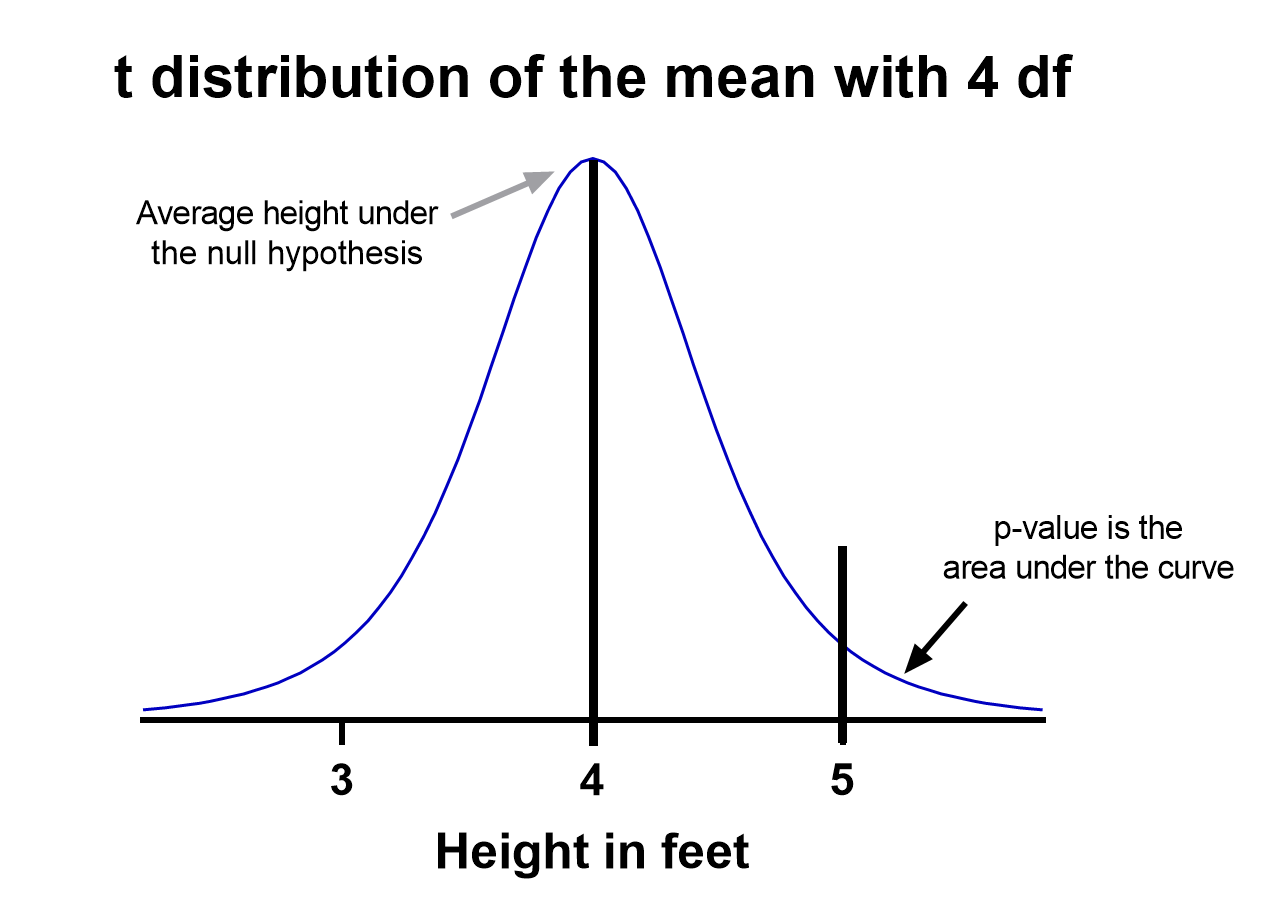
Notice the vertical line at x = 5, which was our sample mean. We (use software to) calculate the area to the right of the vertical line, which gives us the P value (0.09 in this case). Note that because our research question was asking if the average student is greater than four feet, the distribution is centered at four. Since we’re only interested in knowing if the average is greater than four feet, we use a one-tailed test in this case.
Using the standard confidence level of 0.05 with this example, we don’t have evidence that the true average height of sixth graders is taller than 4 feet.
What are the assumptions for t tests?
- One variable of interest : This is not correlation or regression, where you are interested in the relationship between multiple variables. With a t test, you can have different samples, but they are all measuring the same variable (e.g., height).
- Numeric data: You are dealing with a list of measurements that can be averaged. This means you aren’t just counting occurrences in various categories (e.g., eye color or political affiliation).
- Two groups or less: If you have more than two samples of data, a t test is the wrong technique. You most likely need to try ANOVA.
- Random sample : You need a random sample from your statistical “population of interest” in order to draw valid conclusions about the larger population. If your population is so small that you can measure everything, then you have a “census” and don’t need statistics. This is because you don’t need to estimate the truth, since you have measured the truth without variability.
- Normally Distributed : The smaller your sample size, the more important it is that your data come from a normal, Gaussian distribution bell curve. If you have reason to believe that your data are not normally distributed, consider nonparametric t test alternatives . This isn’t necessary for larger samples (usually 25 or 30 unless the data is heavily skewed). The reason is that the Central Limit Theorem applies in this case, which says that even if the distribution of your data is not normal, the distribution of the mean of your data is, so you can use a z-test rather than a t test.
How do I know which t test to use?
There are many types of t tests to choose from, but you don’t necessarily have to understand every detail behind each option.
You just need to be able to answer a few questions, which will lead you to pick the right t test. To that end, we put together this workflow for you to figure out which test is appropriate for your data.
Do you have one or two samples?
Are you comparing the means of two different samples, or comparing the mean from one sample to a fixed value? An example research question is, “Is the average height of my sample of sixth grade students greater than four feet?”
If you only have one sample of data, you can click here to skip to a one-sample t test example, otherwise your next step is to ask:
Are observations in the two samples matched up or related in some way?
This could be as before-and-after measurements of the same exact subjects, or perhaps your study split up “pairs” of subjects (who are technically different but share certain characteristics of interest) into the two samples. The same variable is measured in both cases.
If so, you are looking at some kind of paired samples t test . The linked section will help you dial in exactly which one in that family is best for you, either difference (most common) or ratio.
If you aren’t sure paired is right, ask yourself another question:
Are you comparing different observations in each of the two samples?
If the answer is yes, then you have an unpaired or independent samples t test. The two samples should measure the same variable (e.g., height), but are samples from two distinct groups (e.g., team A and team B).
The goal is to compare the means to see if the groups are significantly different. For example, “Is the average height of team A greater than team B?” Unlike paired, the only relationship between the groups in this case is that we measured the same variable for both. There are two versions of unpaired samples t tests (pooled and unpooled) depending on whether you assume the same variance for each sample.
Have you run the same experiment multiple times on the same subject/observational unit?
If so, then you have a nested t test (unless you have more than two sample groups). This is a trickier concept to understand. One example is if you are measuring how well Fertilizer A works against Fertilizer B. Let’s say you have 12 pots to grow plants in (6 pots for each fertilizer), and you grow 3 plants in each pot.
In this case you have 6 observational units for each fertilizer, with 3 subsamples from each pot. You would want to analyze this with a nested t test . The “nested” factor in this case is the pots. It’s important to note that we aren’t interested in estimating the variability within each pot, we just want to take it into account.
You might be tempted to run an unpaired samples t test here, but that assumes you have 6*3 = 18 replicates for each fertilizer. However, the three replicates within each pot are related, and an unpaired samples t test wouldn’t take that into account.
What if none of these sound like my experiment?
If you’re not seeing your research question above, note that t tests are very basic statistical tools. Many experiments require more sophisticated techniques to evaluate differences. If the variable of interest is a proportion (e.g., 10 of 100 manufactured products were defective), then you’d use z-tests. If you take before and after measurements and have more than one treatment (e.g., control vs a treatment diet), then you need ANOVA.
How do I perform a t test using software?
If you’re wondering how to do a t test, the easiest way is with statistical software such as Prism or an online t test calculator .
If you’re using software, then all you need to know is which t test is appropriate ( use the workflow here ) and understand how to interpret the output. To do that, you’ll also need to:
- Determine whether your test is one or two-tailed
- Choose the level of significance
Is my test one or two-tailed?
Whether or not you have a one- or two-tailed test depends on your research hypothesis. Choosing the appropriately tailed test is very important and requires integrity from the researcher. This is because you have more “power” with one-tailed tests, meaning that you can detect a statistically significant difference more easily. Unless you have written out your research hypothesis as one directional before you run your experiment, you should use a two-tailed test.
Two-tailed tests
Two-tailed tests are the most common, and they are applicable when your research question is simply asking, “is there a difference?”
One-tailed tests
Contrast that with one-tailed tests, where the research questions are directional, meaning that either the question is, “is it greater than ” or the question is, “is it less than ”. These tests can only detect a difference in one direction.
Choosing the level of significance
All t tests estimate whether a mean of a population is different than some other value, and with all estimates come some variability, or what statisticians call “error.” Before analyzing your data, you want to choose a level of significance, usually denoted by the Greek letter alpha, 𝛼. The scientific standard is setting alpha to be 0.05.
An alpha of 0.05 results in 95% confidence intervals, and determines the cutoff for when P values are considered statistically significant.
One sample t test
If you only have one sample of a list of numbers, you are doing a one-sample t test. All you are interested in doing is comparing the mean from this group with some known value to test if there is evidence, that it is significantly different from that standard. Use our free one-sample t test calculator for this.
A one sample t test example research question is, “Is the average fifth grader taller than four feet?”
It is the simplest version of a t test, and has all sorts of applications within hypothesis testing. Sometimes the “known value” is called the “null value”. While the null value in t tests is often 0, it could be any value. The name comes from being the value which exactly represents the null hypothesis, where no significant difference exists.
Any time you know the exact number you are trying to compare your sample of data against, this could work well. And of course: it can be either one or two-tailed.
One sample t test formula
Statistical software handles this for you, but if you want the details, the formula for a one sample t test is:
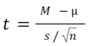
- M: Calculated mean of your sample
- μ: Hypothetical mean you are testing against
- s: The standard deviation of your sample
- n: The number of observations in your sample.
In a one-sample t test, calculating degrees of freedom is simple: one less than the number of objects in your dataset (you’ll see it written as n-1 ).
Example of a one sample t test
For our example within Prism, we have a dataset of 12 values from an experiment labeled “% of control”. Perhaps these are heights of a sample of plants that have been treated with a new fertilizer. A value of 100 represents the industry-standard control height. Likewise, 123 represents a plant with a height 123% that of the control (that is, 23% larger).
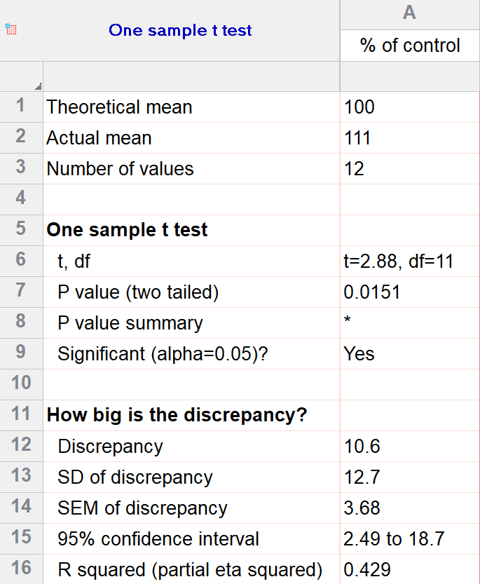
We’ll perform a two-tailed, one-sample t test to see if plants are shorter or taller on average with the fertilizer. We will use a significance threshold of 0.05. Here is the output:
You can see in the output that the actual sample mean was 111. Is that different enough from the industry standard (100) to conclude that there is a statistical difference?
The quick answer is yes, there’s strong evidence that the height of the plants with the fertilizer is greater than the industry standard (p=0.015). The nice thing about using software is that it handles some of the trickier steps for you. In this case, it calculates your test statistic (t=2.88), determines the appropriate degrees of freedom (11), and outputs a P value.
More informative than the P value is the confidence interval of the difference, which is 2.49 to 18.7. The confidence interval tells us that, based on our data, we are confident that the true difference between our sample and the baseline value of 100 is somewhere between 2.49 and 18.7. As long as the difference is statistically significant, the interval will not contain zero.
You can follow these tips for interpreting your own one-sample test.
Graphing a one-sample t test
For some techniques (like regression), graphing the data is a very helpful part of the analysis. For t tests, making a chart of your data is still useful to spot any strange patterns or outliers, but the small sample size means you may already be familiar with any strange things in your data.
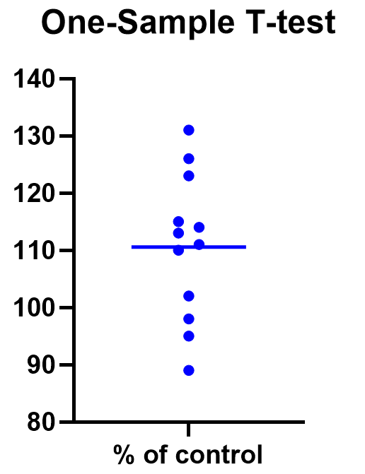
Here we have a simple plot of the data points, perhaps with a mark for the average. We’ve made this as an example, but the truth is that graphing is usually more visually telling for two-sample t tests than for just one sample.
Two sample t tests
There are several kinds of two sample t tests, with the two main categories being paired and unpaired (independent) samples.
Paired samples t test
In a paired samples t test, also called dependent samples t test, there are two samples of data, and each observation in one sample is “paired” with an observation in the second sample. The most common example is when measurements are taken on each subject before and after a treatment. A paired t test example research question is, “Is there a statistical difference between the average red blood cell counts before and after a treatment?”
Having two samples that are closely related simplifies the analysis. Statistical software, such as this paired t test calculator , will simply take a difference between the two values, and then compare that difference to 0.
In some (rare) situations, taking a difference between the pairs violates the assumptions of a t test, because the average difference changes based on the size of the before value (e.g., there’s a larger difference between before and after when there were more to start with). In this case, instead of using a difference test, use a ratio of the before and after values, which is referred to as ratio t tests .
Paired t test formula
The formula for paired samples t test is:
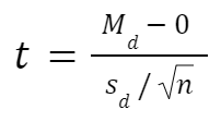
- Md: Mean difference between the samples
- sd: The standard deviation of the differences
- n: The number of differences
Degrees of freedom are the same as before. If you’re studying for an exam, you can remember that the degrees of freedom are still n-1 (not n-2) because we are converting the data into a single column of differences rather than considering the two groups independently.
Also note that the null value here is simply 0. There is no real reason to include “minus 0” in an equation other than to illustrate that we are still doing a hypothesis test. After you take the difference between the two means, you are comparing that difference to 0.
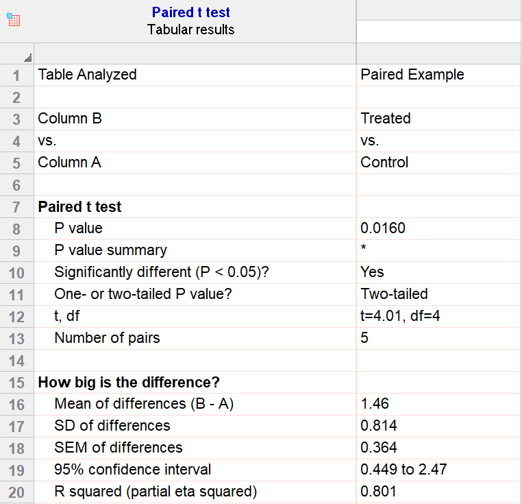
For our example data, we have five test subjects and have taken two measurements from each: before (“control”) and after a treatment (“treated”). If we set alpha = 0.05 and perform a two-tailed test, we observe a statistically significant difference between the treated and control group (p=0.0160, t=4.01, df = 4). We are 95% confident that the true mean difference between the treated and control group is between 0.449 and 2.47.
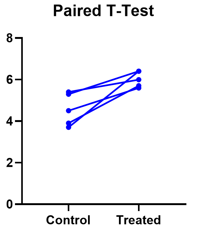
Graphing a paired t test
The significant result of the P value suggests evidence that the treatment had some effect, and we can also look at this graphically. The lines that connect the observations can help us spot a pattern, if it exists. In this case the lines show that all observations increased after treatment. While not all graphics are this straightforward, here it is very consistent with the outcome of the t test.
Prism’s estimation plot is even more helpful because it shows both the data (like above) and the confidence interval for the difference between means. You can easily see the evidence of significance since the confidence interval on the right does not contain zero.
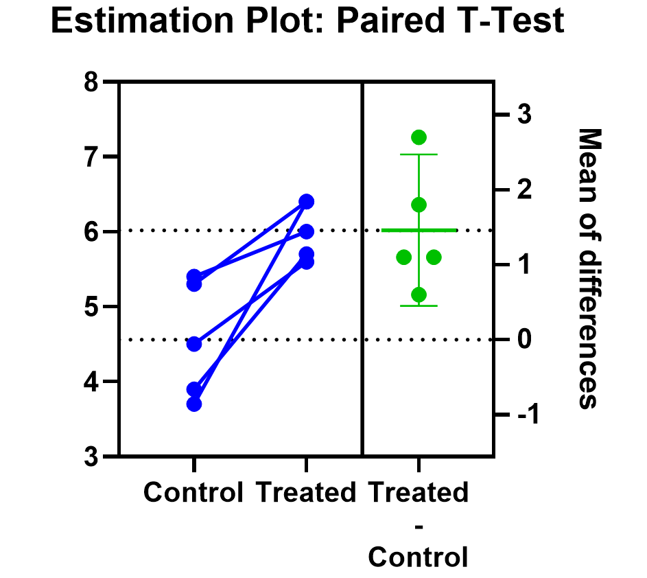
Here are some more graphing tips for paired t tests .
Unpaired samples t test
Unpaired samples t test, also called independent samples t test, is appropriate when you have two sample groups that aren’t correlated with one another. A pharma example is testing a treatment group against a control group of different subjects. Compare that with a paired sample, which might be recording the same subjects before and after a treatment.
With unpaired t tests, in addition to choosing your level of significance and a one or two tailed test, you need to determine whether or not to assume that the variances between the groups are the same or not. If you assume equal variances, then you can “pool” the calculation of the standard error between the two samples. Otherwise, the standard choice is Welch’s t test which corrects for unequal variances. This choice affects the calculation of the test statistic and the power of the test, which is the test’s sensitivity to detect statistical significance.
It’s best to choose whether or not you’ll use a pooled or unpooled (Welch’s) standard error before running your experiment, because the standard statistical test is notoriously problematic. See more details about unequal variances here .
As long as you’re using statistical software, such as this two-sample t test calculator , it’s just as easy to calculate a test statistic whether or not you assume that the variances of your two samples are the same. If you’re doing it by hand, however, the calculations get more complicated with unequal variances.
Unpaired (independent) samples t test formula
The general two-sample t test formula is:
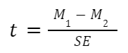
- M1 and M2: Two means you are comparing, one from each dataset
- SE : The combined standard error of the two samples (calculated using pooled or unpooled standard error)
The denominator (standard error) calculation can be complicated, as can the degrees of freedom. If the groups are not balanced (the same number of observations in each), you will need to account for both when determining n for the test as a whole.
As an example for this family, we conduct a paired samples t test assuming equal variances (pooled). Based on our research hypothesis, we’ll conduct a two-tailed test, and use alpha=0.05 for our level of significance. Our samples were unbalanced, with two samples of 6 and 5 observations respectively.
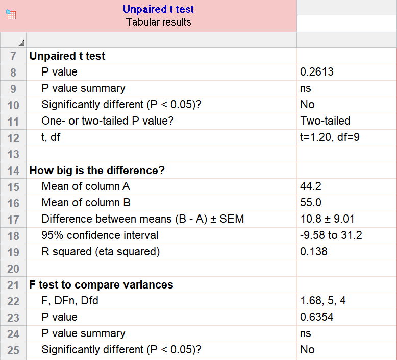
The P value (p=0.261, t = 1.20, df = 9) is higher than our threshold of 0.05. We have not found sufficient evidence to suggest a significant difference. You can see the confidence interval of the difference of the means is -9.58 to 31.2.
Note that the F-test result shows that the variances of the two groups are not significantly different from each other.
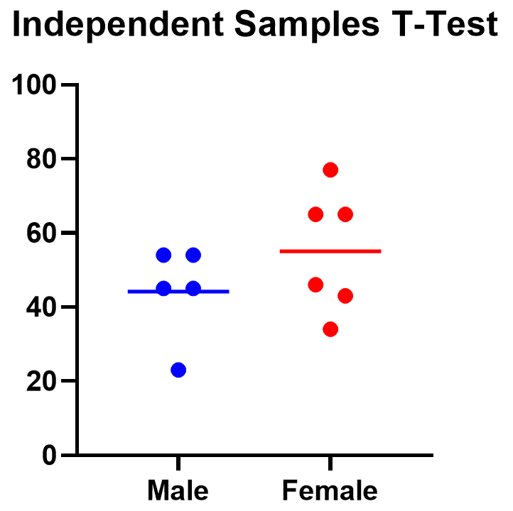
Graphing an unpaired samples t test
For an unpaired samples t test, graphing the data can quickly help you get a handle on the two groups and how similar or different they are. Like the paired example, this helps confirm the evidence (or lack thereof) that is found by doing the t test itself.
Below you can see that the observed mean for females is higher than that for males. But because of the variability in the data, we can’t tell if the means are actually different or if the difference is just by chance.
Nonparametric alternatives for t tests
If your data comes from a normal distribution (or something close enough to a normal distribution), then a t test is valid. If that assumption is violated, you can use nonparametric alternatives.
T tests evaluate whether the mean is different from another value, whereas nonparametric alternatives compare either the median or the rank. Medians are well-known to be much more robust to outliers than the mean.
The downside to nonparametric tests is that they don’t have as much statistical power, meaning a larger difference is required in order to determine that it’s statistically significant.
Wilcoxon signed-rank test
The Wilcoxon signed-rank test is the nonparametric cousin to the one-sample t test. This compares a sample median to a hypothetical median value. It is sometimes erroneously even called the Wilcoxon t test (even though it calculates a “W” statistic).
And if you have two related samples, you should use the Wilcoxon matched pairs test instead. The two versions of Wilcoxon are different, and the matched pairs version is specifically for comparing the median difference for paired samples.
Mann-Whitney and Kolmogorov-Smirnov tests
For unpaired (independent) samples, there are multiple options for nonparametric testing. Mann-Whitney is more popular and compares the mean ranks (the ordering of values from smallest to largest) of the two samples. Mann-Whitney is often misrepresented as a comparison of medians, but that’s not always the case. Kolmogorov-Smirnov tests if the overall distributions differ between the two samples.
More t test FAQs
What is the formula for a t test.
The exact formula depends on which type of t test you are running, although there is a basic structure that all t tests have in common. All t test statistics will have the form:
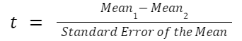
- t : The t test statistic you calculate for your test
- Mean1 and Mean2: Two means you are comparing, at least 1 from your own dataset
- Standard Error of the Mean : The standard error of the mean , also called the standard deviation of the mean, which takes into account the variance and size of your dataset
The exact formula for any t test can be slightly different, particularly the calculation of the standard error. Not only does it matter whether one or two samples are being compared, the relationship between the samples can make a difference too.
What is a t-distribution?
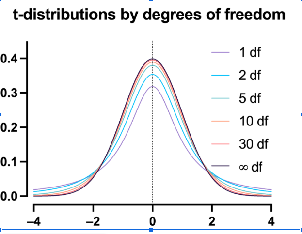
A t-distribution is similar to a normal distribution. It’s a bell-shaped curve, but compared to a normal it has fatter tails, which means that it’s more common to observe extremes. T-distributions are identified by the number of degrees of freedom. The higher the number, the closer the t-distribution gets to a normal distribution. After about 30 degrees of freedom, a t and a standard normal are practically the same.
What are degrees of freedom?
Degrees of freedom are a measure of how large your dataset is. They aren’t exactly the number of observations, because they also take into account the number of parameters (e.g., mean, variance) that you have estimated.
What is the difference between paired vs unpaired t tests?
Both paired and unpaired t tests involve two sample groups of data. With a paired t test, the values in each group are related (usually they are before and after values measured on the same test subject). In contrast, with unpaired t tests, the observed values aren’t related between groups. An unpaired, or independent t test, example is comparing the average height of children at school A vs school B.
When do I use a z-test versus a t test?
Z-tests, which compare data using a normal distribution rather than a t-distribution, are primarily used for two situations. The first is when you’re evaluating proportions (number of failures on an assembly line). The second is when your sample size is large enough (usually around 30) that you can use a normal approximation to evaluate the means.
When should I use ANOVA instead of a t test?
Use ANOVA if you have more than two group means to compare.
What are the differences between t test vs chi square?
Chi square tests are used to evaluate contingency tables , which record a count of the number of subjects that fall into particular categories (e.g., truck, SUV, car). t tests compare the mean(s) of a variable of interest (e.g., height, weight).
What are P values?
P values are the probability that you would get data as or more extreme than the observed data given that the null hypothesis is true. It’s a mouthful, and there are a lot of issues to be aware of with P values.
What are t test critical values?
Critical values are a classical form (they aren’t used directly with modern computing) of determining if a statistical test is significant or not. Historically you could calculate your test statistic from your data, and then use a t-table to look up the cutoff value (critical value) that represented a “significant” result. You would then compare your observed statistic against the critical value.
How do I calculate degrees of freedom for my t test?
In most practical usage, degrees of freedom are the number of observations you have minus the number of parameters you are trying to estimate. The calculation isn’t always straightforward and is approximated for some t tests.
Statistical software calculates degrees of freedom automatically as part of the analysis, so understanding them in more detail isn’t needed beyond assuaging any curiosity.
Perform your own t test
Are you ready to calculate your own t test? Start your 30 day free trial of Prism and get access to:
- A step by step guide on how to perform a t test
- Sample data to save you time
- More tips on how Prism can help your research
With Prism, in a matter of minutes you learn how to go from entering data to performing statistical analyses and generating high-quality graphs.
JMP | Statistical Discovery.™ From SAS.
Statistics Knowledge Portal
A free online introduction to statistics
What is a t- test?
A t -test (also known as Student's t -test) is a tool for evaluating the means of one or two populations using hypothesis testing. A t-test may be used to evaluate whether a single group differs from a known value (a one-sample t-test), whether two groups differ from each other (an independent two-sample t-test), or whether there is a significant difference in paired measurements (a paired, or dependent samples t-test).
How are t -tests used?
First, you define the hypothesis you are going to test and specify an acceptable risk of drawing a faulty conclusion. For example, when comparing two populations, you might hypothesize that their means are the same, and you decide on an acceptable probability of concluding that a difference exists when that is not true. Next, you calculate a test statistic from your data and compare it to a theoretical value from a t- distribution. Depending on the outcome, you either reject or fail to reject your null hypothesis.
What if I have more than two groups?
You cannot use a t -test. Use a multiple comparison method. Examples are analysis of variance ( ANOVA ) , Tukey-Kramer pairwise comparison, Dunnett's comparison to a control, and analysis of means (ANOM).
t -Test assumptions
While t -tests are relatively robust to deviations from assumptions, t -tests do assume that:
- The data are continuous.
- The sample data have been randomly sampled from a population.
- There is homogeneity of variance (i.e., the variability of the data in each group is similar).
- The distribution is approximately normal.
For two-sample t -tests, we must have independent samples. If the samples are not independent, then a paired t -test may be appropriate.
Types of t -tests
There are three t -tests to compare means: a one-sample t -test, a two-sample t -test and a paired t -test. The table below summarizes the characteristics of each and provides guidance on how to choose the correct test. Visit the individual pages for each type of t -test for examples along with details on assumptions and calculations.
| test | test | test | |
|---|---|---|---|
| Synonyms | Student’s -test | -test test -test -test -test | test -test |
| Number of variables | One | Two | Two |
| Type of variable | |||
| Purpose of test | Decide if the population mean is equal to a specific value or not | Decide if the population means for two different groups are equal or not | Decide if the difference between paired measurements for a population is zero or not |
| Example: test if... | Mean heart rate of a group of people is equal to 65 or not | Mean heart rates for two groups of people are the same or not | Mean difference in heart rate for a group of people before and after exercise is zero or not |
| Estimate of population mean | Sample average | Sample average for each group | Sample average of the differences in paired measurements |
| Population standard deviation | Unknown, use sample standard deviation | Unknown, use sample standard deviations for each group | Unknown, use sample standard deviation of differences in paired measurements |
| Degrees of freedom | Number of observations in sample minus 1, or: n–1 | Sum of observations in each sample minus 2, or: n + n – 2 | Number of paired observations in sample minus 1, or: n–1 |
The table above shows only the t -tests for population means. Another common t -test is for correlation coefficients . You use this t -test to decide if the correlation coefficient is significantly different from zero.
One-tailed vs. two-tailed tests
When you define the hypothesis, you also define whether you have a one-tailed or a two-tailed test. You should make this decision before collecting your data or doing any calculations. You make this decision for all three of the t -tests for means.
To explain, let’s use the one-sample t -test. Suppose we have a random sample of protein bars, and the label for the bars advertises 20 grams of protein per bar. The null hypothesis is that the unknown population mean is 20. Suppose we simply want to know if the data shows we have a different population mean. In this situation, our hypotheses are:
$ \mathrm H_o: \mu = 20 $
$ \mathrm H_a: \mu \neq 20 $
Here, we have a two-tailed test. We will use the data to see if the sample average differs sufficiently from 20 – either higher or lower – to conclude that the unknown population mean is different from 20.
Suppose instead that we want to know whether the advertising on the label is correct. Does the data support the idea that the unknown population mean is at least 20? Or not? In this situation, our hypotheses are:
$ \mathrm H_o: \mu >= 20 $
$ \mathrm H_a: \mu < 20 $
Here, we have a one-tailed test. We will use the data to see if the sample average is sufficiently less than 20 to reject the hypothesis that the unknown population mean is 20 or higher.
See the "tails for hypotheses tests" section on the t -distribution page for images that illustrate the concepts for one-tailed and two-tailed tests.
How to perform a t -test
For all of the t -tests involving means, you perform the same steps in analysis:
- Define your null ($ \mathrm H_o $) and alternative ($ \mathrm H_a $) hypotheses before collecting your data.
- Decide on the alpha value (or α value). This involves determining the risk you are willing to take of drawing the wrong conclusion. For example, suppose you set α=0.05 when comparing two independent groups. Here, you have decided on a 5% risk of concluding the unknown population means are different when they are not.
- Check the data for errors.
- Check the assumptions for the test.
- Perform the test and draw your conclusion. All t -tests for means involve calculating a test statistic. You compare the test statistic to a theoretical value from the t- distribution . The theoretical value involves both the α value and the degrees of freedom for your data. For more detail, visit the pages for one-sample t -test , two-sample t -test and paired t -test .
Uncomplicated Reviews of Educational Research Methods
- Significance Testing (t-tests)
.pdf version of this page
In this review, we’ll look at significance testing, using mostly the t -test as a guide. As you read educational research, you’ll encounter t -test and ANOVA statistics frequently. Part I reviews the basics of significance testing as related to the null hypothesis and p values. Part II shows you how to conduct a t -test, using an online calculator. Part III deal s with interpreting t -test results. Part IV is about reporting t -test results in both text and table formats and concludes with a guide to interpreting confidence intervals.
What is Statistical Significance?
The terms “significance level” or “level of significance” refer to the likelihood that the random sample you choose (for example, test scores) is not representative of the population. The lower the significance level, the more confident you can be in replicating your results. Significance levels most commonly used in educational research are the .05 and .01 levels. If it helps, think of .05 as another way of saying 95/100 times that you sample from the population, you will get this result. Similarly, .01 suggests that 99/100 times that you sample from the population, you will get the same result. These numbers and signs (more on that later) come from Significance Testing, which begins with the Null Hypothesis.
Part I: The Null Hypothesis
We start by revisiting familiar territory, the scientific method . We’ll start with a basic research question: How does variable A affect variable B? The traditional way to test this question involves:
Step 1. Develop a research question.
Step 2. Find previous research to support, refute, or suggest ways of testing the question.
Step 3. Construct a hypothesis by revising your research question:
| H1: A = B | There is no relationship between A and B | Null |
| H2: A ≠ B | There is a relationship between A and B. Here, there is a relationship, but we don’t know if it is positive or negative. | Alternate |
| H3: A < B | There is a negative relationship between A and B. Here, the < suggests that the less A is involved, the better B. | Alternate |
| H4: A > B | There is a positive relationship between A and B. Here, the > suggests that the more B is involved, the better A. | Alternate |
Step 4. Test the null hypothesis. To test the null hypothesis, A = B, we use a significance test. The italicized lowercase p you often see, followed by > or < sign and a decimal ( p ≤ .05) indicate significance. In most cases, the researcher tests the null hypothesis, A = B , because is it easier to show there is some sort of effect of A on B, than to have to determine a positive or negative effect prior to conducting the research. This way, you leave yourself room without having the burden of proof on your study from the beginning.
Step 5. Analyze data and draw a conclusion. Testing the null hypothesis leaves two possibilities:
| A = B | Fail to reject the null. We find no relationship between A and B. | Null |
| A =, <, or > B | Reject the null. We find a relationship between A and B. | Alternate |
Step 6. Communicate results. See Wording results, below.
Part II: Conducting a t -test (for Independent Means)
So how do we test a null hypothesis? One way is with a t -test. A t -test asks the question,
“Is the difference between the means of two samples different (significant) enough to say that some other characteristic (teaching method, teacher, gender, etc.) could have caused it?”
To conduct a t-test using an online calculator, complete the following steps:
Step 1. Compose the Research Question.
Step 2. Compose a Null and an Alternative Hypothesis.
Step 3. Obtain two random samples of at least 30, preferably 50, from each group.
Step 4. Conduct a t -test:
- Go to http://www.graphpad.com/quickcalcs/ttest1.cfm
- For #1, check “Enter mean, SD and N.”
- For #2, label your groups and enter data. You will need to have mean and SD. N is group size.
- For #3, check “Unpaired t test.”
- For #4, click “Calculate now.”
Step 5. Interpret the results (see below).
Step 6. Report results in text or table format (see below).
- Get p from “P value and statistical significance:” Note that this is the actual value.
- Get the confidence interval from “Confidence interval:”
- Get the t and df values from “Intermediate values used in calculations:”
- Get Mean , and SD from “Review your data.”
Part III. Interpreting a t-test (Understanding the Numbers)
| tells you a test was used. | |
| (98) | tells you the (the sample of tests performed). |
| 3.09 | is the “ statistic” – the result of the calculation. |
| ≤ .05 | is the probability of getting the observed score from the sample groups. |
| .05 | likely to be a result of chance (same as saying A = B) |
| difference is not significant | |
| null is correct | |
| “fail to reject the null” | |
| There is no relationship between A and B. | |
| ≤ .05 | not likely to be a result of chance (same as saying A ≠ B) |
| difference is significant | |
| null is incorrect | |
| “reject the null” | |
| There is a relationship between A and B. |
Note: We acknowledge that the average scores are different. With a t -test we are deciding if that difference is significant (is it due to sampling error or something else?).
Understanding the Confidence Interval (CI)
The Confidence Interval (CI) of a mean is a region within which a score (like mean test score) may be said to fall with a certain amount of “confidence.” The CI uses sample size and standard deviation to generate a lower and upper number that you can be 95% sure will include any sample you take from a set of data.
Consider Georgia’s AYP measure, the CRCT . For a science CRCT score, we take several samples and compare the different means. After a few calculations, we could determine something like. . .the average difference (mean) between samples is -7.5, with a 95% CI of -22.08 to 6.72. In other words, among all students’ science CRCT scores, 95 out of 100 times we take group samples for comparison (for example by year, or gender, etc.), one of the groups, on average will be 7.5 points lower than the other group. We can be fairly certain that the difference in scores will be between -22.08 and 6.72 points.
Part IV. Wording Results
Wording Results in Text
In text, the basic format is to report: population ( N ), mean ( M ) and standard deviation ( SD ) for both samples, t value, degrees freedom ( df ), significance ( p ), and confidence interval (CI .95 )* .
Example 1: p ≤ .05, or Significant Results
Among 7th graders in Lowndes County Schools taking the CRCT reading exam ( N = 336), there was a statistically significant difference between the two teaching teams, team 1 ( M = 818.92, SD = 16.11) and team 2 ( M = 828.28, SD = 14.09), t (98) = 3.09, p ≤ .05, CI .95 -15.37, -3.35. Therefore, we reject the null hypothesis that there is no difference in reading scores between teaching teams 1 and 2.
Example 2: p ≥ .05, or Not Significant Results
Among 7th graders in Lowndes County Schools taking the CRCT science exam ( N = 336), there was no statistically significant difference between female students (M = 834.00, SD = 32.81) and male students (841.08, SD = 28.76), t (98) = 1.15 p ≥ .05, CI .95 -19.32, 5.16. Therefore, we fail to reject the null hypothesis that there is no difference in science scores between females and males.
Wording Results in APA Table Format
Table 1. Comparison of CRCT 7 th Grade Science Scores by Gender
|
|
|
|
|
|
|
| |
| Female |
50
|
834.00 |
32.81 |
– |
– |
– |
– |
| Male |
50
|
841.08 |
28.76 |
– |
– |
– |
– |
| Total |
100
|
837.54 |
30.90 |
1.14 |
98 |
.2540 |
-19.32 – 5.16 |
Note: On the Web site, this appears blocked and should not be. See the .pdf for the correct format.
Share this:
About research rundowns.
Research Rundowns was made possible by support from the Dewar College of Education at Valdosta State University .
- Experimental Design
- What is Educational Research?
- Writing Research Questions
- Mixed Methods Research Designs
- Qualitative Coding & Analysis
- Qualitative Research Design
- Correlation
- Effect Size
- Instrument, Validity, Reliability
- Mean & Standard Deviation
- Steps 1-4: Finding Research
- Steps 5-6: Analyzing & Organizing
- Steps 7-9: Citing & Writing
- Writing a Research Report
Create a free website or blog at WordPress.com.
- Already have a WordPress.com account? Log in now.
- Subscribe Subscribed
- Copy shortlink
- Report this content
- View post in Reader
- Manage subscriptions
- Collapse this bar
- Skip to secondary menu
- Skip to main content
- Skip to primary sidebar
Statistics By Jim
Making statistics intuitive
How t-Tests Work: t-Values, t-Distributions, and Probabilities
By Jim Frost 12 Comments
T-tests are statistical hypothesis tests that you use to analyze one or two sample means. Depending on the t-test that you use, you can compare a sample mean to a hypothesized value, the means of two independent samples, or the difference between paired samples. In this post, I show you how t-tests use t-values and t-distributions to calculate probabilities and test hypotheses.
As usual, I’ll provide clear explanations of t-values and t-distributions using concepts and graphs rather than formulas! If you need a primer on the basics, read my hypothesis testing overview .
What Are t-Values?
The term “t-test” refers to the fact that these hypothesis tests use t-values to evaluate your sample data. T-values are a type of test statistic. Hypothesis tests use the test statistic that is calculated from your sample to compare your sample to the null hypothesis. If the test statistic is extreme enough, this indicates that your data are so incompatible with the null hypothesis that you can reject the null. Learn more about Test Statistics .

Don’t worry. I find these technical definitions of statistical terms are easier to explain with graphs, and we’ll get to that!
When you analyze your data with any t-test, the procedure reduces your entire sample to a single value, the t-value. These calculations factor in your sample size and the variation in your data. Then, the t-test compares your sample means(s) to the null hypothesis condition in the following manner:
- If the sample data equals the null hypothesis precisely, the t-test produces a t-value of 0.
- As the sample data become progressively dissimilar from the null hypothesis, the absolute value of the t-value increases.
Read the companion post where I explain how t-tests calculate t-values .
The tricky thing about t-values is that they are a unitless statistic, which makes them difficult to interpret on their own. Imagine that we performed a t-test, and it produced a t-value of 2. What does this t-value mean exactly? We know that the sample mean doesn’t equal the null hypothesis value because this t-value doesn’t equal zero. However, we don’t know how exceptional our value is if the null hypothesis is correct.
To be able to interpret individual t-values, we have to place them in a larger context. T-distributions provide this broader context so we can determine the unusualness of an individual t-value.
What Are t-Distributions?
A single t-test produces a single t-value. Now, imagine the following process. First, let’s assume that the null hypothesis is true for the population. Now, suppose we repeat our study many times by drawing many random samples of the same size from this population. Next, we perform t-tests on all of the samples and plot the distribution of the t-values. This distribution is known as a sampling distribution, which is a type of probability distribution.
Related posts : Sampling Distributions and Understanding Probability Distributions
If we follow this procedure, we produce a graph that displays the distribution of t-values that we obtain from a population where the null hypothesis is true. We use sampling distributions to calculate probabilities for how unusual our sample statistic is if the null hypothesis is true.

Luckily, we don’t need to go through the hassle of collecting numerous random samples to create this graph! Statisticians understand the properties of t-distributions so we can estimate the sampling distribution using the t-distribution and our sample size.
The degrees of freedom (DF) for the statistical design define the t-distribution for a particular study. The DF are closely related to the sample size. For t-tests, there is a different t-distribution for each sample size.
Related posts : Degrees of Freedom in Statistics and T Distribution: Definition and Uses .
Use the t-Distribution to Compare Your Sample Results to the Null Hypothesis
T-distributions assume that the null hypothesis is correct for the population from which you draw your random samples. To evaluate how compatible your sample data are with the null hypothesis, place your study’s t-value in the t-distribution and determine how unusual it is.
The sampling distribution below displays a t-distribution with 20 degrees of freedom, which equates to a sample size of 21 for a 1-sample t-test. The t-distribution centers on zero because it assumes that the null hypothesis is true. When the null is true, your study is most likely to obtain a t-value near zero and less liable to produce t-values further from zero in either direction.

On the graph, I’ve displayed the t-value of 2 from our hypothetical study to see how our sample data compares to the null hypothesis. Under the assumption that the null is true, the t-distribution indicates that our t-value is not the most likely value. However, there still appears to be a realistic chance of observing t-values from -2 to +2.
We know that our t-value of 2 is rare when the null hypothesis is true. How rare is it exactly? Our final goal is to evaluate whether our sample t-value is so rare that it justifies rejecting the null hypothesis for the entire population based on our sample data. To proceed, we need to quantify the probability of observing our t-value.
Related post : What are Critical Values?
t-Tests Use t-Values and t-Distributions to Calculate Probabilities
Hypothesis tests work by taking the observed test statistic from a sample and using the sampling distribution to calculate the probability of obtaining that test statistic if the null hypothesis is correct. In the context of how t-tests work, you assess the likelihood of a t-value using the t-distribution. If a t-value is sufficiently improbable when the null hypothesis is true, you can reject the null hypothesis.
I have two crucial points to explain before we calculate the probability linked to our t-value of 2.
Because I’m showing the results of a two-tailed test, we’ll use the t-values of +2 and -2. Two-tailed tests allow you to assess whether the sample mean is greater than or less than the target value in a 1-sample t-test. A one-tailed hypothesis test can only determine statistical significance for one or the other.
Additionally, it is possible to calculate a probability only for a range of t-values. On a probability distribution plot, probabilities are represented by the shaded area under a distribution curve. Without a range of values, there is no area under the curve and, hence, no probability.
Related posts : One-Tailed and Two-Tailed Tests Explained and T-Distribution Table of Critical Values
t-Test Results for Our Hypothetical Study
Considering these points, the graph below finds the probability associated with t-values less than -2 and greater than +2 using the area under the curve. This graph is specific to our t-test design (1-sample t-test with N = 21).

The probability distribution plot indicates that each of the two shaded regions has a probability of 0.02963—for a total of 0.05926. This graph shows that t-values fall within these areas almost 6% of the time when the null hypothesis is true.
There is a chance that you’ve heard of this type of probability before—it’s the P value! While the likelihood of t-values falling within these regions seems small, it’s not quite unlikely enough to justify rejecting the null under the standard significance level of 0.05.
Learn how to interpret the P value correctly and avoid a common mistake!
Related posts : How to Find the P value: Process and Calculations and Types of Errors in Hypothesis Testing
t-Distributions and Sample Size
The sample size for a t-test determines the degrees of freedom (DF) for that test, which specifies the t-distribution. The overall effect is that as the sample size decreases, the tails of the t-distribution become thicker. Thicker tails indicate that t-values are more likely to be far from zero even when the null hypothesis is correct. The changing shapes are how t-distributions factor in the greater uncertainty when you have a smaller sample.
You can see this effect in the probability distribution plot below that displays t-distributions for 5 and 30 DF.

Sample means from smaller samples tend to be less precise. In other words, with a smaller sample, it’s less surprising to have an extreme t-value, which affects the probabilities and p-values. A t-value of 2 has a P value of 10.2% and 5.4% for 5 and 30 DF, respectively. Use larger samples!
Click here for step-by-step instructions for how to do t-tests in Excel !
If you like this approach and want to learn about other hypothesis tests, read my posts about:
- How the F-test Works in ANOVA .
- How Chi-Squared Tests of Independence Work
To see an alternative to traditional hypothesis testing that does not use probability distributions and test statistics, learn about bootstrapping in statistics !
Share this:

Reader Interactions

May 25, 2021 at 10:42 pm
what statistical tools, is recommended for measuring the level of satisfaction

May 26, 2021 at 3:55 pm
Hi McKienze,
The correct analysis depends on the nature of the data you have and what you want to learn. You don’t provide enough information to be able to answer the question. However, read my hypothesis testing overview to learn about the options.

August 23, 2020 at 1:33 am
Hi Jim, I want to ask about standardizing data before the t test.. For example I have USD prices of a big Mac across the world and this varies by quite a bit. Doing the t-test here would be misleading since some countries would have a higher mean… Should the approach be standardizing all the usd values? Or perhaps even local values?
August 24, 2020 at 12:37 am
Yes, that makes complete sense. I don’t know what method is best. If you can find a common scale to use for all prices, I’d do that. You’re basically using a data transformation before analysis, which is totally acceptable when you have a good reason.

April 3, 2020 at 4:47 am
Hey Jim. Your blog is one of the only few ones where everything is explained in a simple and well structured manner, in a way that both an absolute beginner and a geek can equally benefit from your writing. Both this article as well as your article on one tailed and two tailed hypothesis tests have been super helpful. Thank you for this post

March 6, 2020 at 11:04 am
Thank you, Jim, for sharing your knowledge with us.
I have a 2 part question. I am testing the difference in walking distance within a busy environment compared with a simple environment. I am also testing walking time within the 2 environments. I am using the same individuals for both scenarios. I was planning to do a paired ttest for distance difference between busy and simple environments and a 2nd paired ttest for time difference between the environments.
My question(s) for you is: 1. Do you feel that a paired ttest is the best choice for these? 2. Do you feel that, because there are 2 tests, I should do a bonferroni correction or do you believe that because the data is completely different (distance as opposed to time), it is okay not to do a multiple comparison test?

August 13, 2019 at 12:43 pm
thank you very eye opening on the use of two or one tailed test

April 19, 2019 at 3:49 pm
Hi Mr. Frost,
Thanks for the breakdown. I have a question … if I wanted to run a test to show that the medical professionals could use more training with data set consisting of questions which in your opinion would be my best route?

January 14, 2019 at 2:22 pm
Hello Jim, I find this statement in this excellent write up contradicting : 1)This graph shows that t-values fall within these areas almost 6% of the time when the null hypothesis is true I mean if this is true the t-value =0 hypothesis is rejected.
January 14, 2019 at 2:51 pm
I can see how that statement sounds contradictory, but I can assure that it is quite accurate. It’s often forgotten but the underlying assumption for the calculations surrounding hypothesis testing, significance levels, and p-values is that the null hypothesis is true.
So, the probabilities shown in the graph that you refer to are based on the assumption that the null hypothesis is true. Further, t-values for this study design have a 6% chance of falling in those critical areas assuming the null is true (a false positive).
Significance levels are defined as the maximum acceptable probability of a false positive. Usually, we set that as 5%. In the example, there’s a large probability of a false positive (6%), so we fail to reject the null hypothesis. In other words, we fail to reject the null because false positives will happen too frequently–where the significance level defines the cutoff point for too frequently.
Keep in mind that when you have statistically significant results, you’re really saying that the results you obtained are improbable enough assuming that the null is true that you can reject the notion that the null is true. But, the math and probabilities are all based on the assumption that the null is true because you need to determine how unlikely your results are under the null hypothesis.
Even the p-value is defined in terms of assuming the null hypothesis is true. You can read about that in my post about interpreting p-values correctly .
I hope this clarifies things!
November 9, 2018 at 2:36 am
Jim …I was involved in in a free SAT/ACT tutoring program that I need to analyze for effectiveness .
I have pre test scores of a number of students and the post test scores after they were tutored (treatment ).
Glenn dowell
November 9, 2018 at 9:05 am
It sounds like you need to perform a paired t-test assuming.
Comments and Questions Cancel reply

- Quality Improvement
- Talk To Minitab
Understanding t-Tests: t-values and t-distributions
Topics: Hypothesis Testing , Data Analysis
T-tests are handy hypothesis tests in statistics when you want to compare means. You can compare a sample mean to a hypothesized or target value using a one-sample t-test. You can compare the means of two groups with a two-sample t-test. If you have two groups with paired observations (e.g., before and after measurements), use the paired t-test.

How do t-tests work? How do t-values fit in? In this series of posts, I’ll answer these questions by focusing on concepts and graphs rather than equations and numbers. After all, a key reason to use statistical software like Minitab is so you don’t get bogged down in the calculations and can instead focus on understanding your results.
In this post, I will explain t-values, t-distributions, and how t-tests use them to calculate probabilities and assess hypotheses.
What Are t-Values?
T-tests are called t-tests because the test results are all based on t-values. T-values are an example of what statisticians call test statistics. A test statistic is a standardized value that is calculated from sample data during a hypothesis test. The procedure that calculates the test statistic compares your data to what is expected under the null hypothesis .
Each type of t-test uses a specific procedure to boil all of your sample data down to one value, the t-value. The calculations behind t-values compare your sample mean(s) to the null hypothesis and incorporates both the sample size and the variability in the data. A t-value of 0 indicates that the sample results exactly equal the null hypothesis. As the difference between the sample data and the null hypothesis increases, the absolute value of the t-value increases.
Assume that we perform a t-test and it calculates a t-value of 2 for our sample data. What does that even mean? I might as well have told you that our data equal 2 fizbins! We don’t know if that’s common or rare when the null hypothesis is true.
By itself, a t-value of 2 doesn’t really tell us anything. T-values are not in the units of the original data, or anything else we’d be familiar with. We need a larger context in which we can place individual t-values before we can interpret them. This is where t-distributions come in.
What Are t-Distributions?
When you perform a t-test for a single study, you obtain a single t-value. However, if we drew multiple random samples of the same size from the same population and performed the same t-test, we would obtain many t-values and we could plot a distribution of all of them. This type of distribution is known as a sampling distribution .
Fortunately, the properties of t-distributions are well understood in statistics, so we can plot them without having to collect many samples! A specific t-distribution is defined by its degrees of freedom (DF) , a value closely related to sample size. Therefore, different t-distributions exist for every sample size. You can graph t-distributions u sing Minitab’s probability distribution plots .
T-distributions assume that you draw repeated random samples from a population where the null hypothesis is true. You place the t-value from your study in the t-distribution to determine how consistent your results are with the null hypothesis.

The graph above shows a t-distribution that has 20 degrees of freedom, which corresponds to a sample size of 21 in a one-sample t-test. It is a symmetric, bell-shaped distribution that is similar to the normal distribution, but with thicker tails. This graph plots the probability density function (PDF), which describes the likelihood of each t-value.
The peak of the graph is right at zero, which indicates that obtaining a sample value close to the null hypothesis is the most likely. That makes sense because t-distributions assume that the null hypothesis is true. T-values become less likely as you get further away from zero in either direction. In other words, when the null hypothesis is true, you are less likely to obtain a sample that is very different from the null hypothesis.
Our t-value of 2 indicates a positive difference between our sample data and the null hypothesis. The graph shows that there is a reasonable probability of obtaining a t-value from -2 to +2 when the null hypothesis is true. Our t-value of 2 is an unusual value, but we don’t know exactly how unusual. Our ultimate goal is to determine whether our t-value is unusual enough to warrant rejecting the null hypothesis. To do that, we'll need to calculate the probability.
Ready for a demo of Minitab Statistical Software? Just ask!

Using t-Values and t-Distributions to Calculate Probabilities
The foundation behind any hypothesis test is being able to take the test statistic from a specific sample and place it within the context of a known probability distribution. For t-tests, if you take a t-value and place it in the context of the correct t-distribution, you can calculate the probabilities associated with that t-value.
A probability allows us to determine how common or rare our t-value is under the assumption that the null hypothesis is true. If the probability is low enough, we can conclude that the effect observed in our sample is inconsistent with the null hypothesis. The evidence in the sample data is strong enough to reject the null hypothesis for the entire population.
Before we calculate the probability associated with our t-value of 2, there are two important details to address.
First, we’ll actually use the t-values of +2 and -2 because we’ll perform a two-tailed test. A two-tailed test is one that can test for differences in both directions. For example, a two-tailed 2-sample t-test can determine whether the difference between group 1 and group 2 is statistically significant in either the positive or negative direction. A one-tailed test can only assess one of those directions.
Second, we can only calculate a non-zero probability for a range of t-values. As you’ll see in the graph below, a range of t-values corresponds to a proportion of the total area under the distribution curve, which is the probability. The probability for any specific point value is zero because it does not produce an area under the curve.
With these points in mind, we’ll shade the area of the curve that has t-values greater than 2 and t-values less than -2.

The graph displays the probability for observing a difference from the null hypothesis that is at least as extreme as the difference present in our sample data while assuming that the null hypothesis is actually true. Each of the shaded regions has a probability of 0.02963, which sums to a total probability of 0.05926. When the null hypothesis is true, the t-value falls within these regions nearly 6% of the time.
This probability has a name that you might have heard of—it’s called the p-value! While the probability of our t-value falling within these regions is fairly low, it’s not low enough to reject the null hypothesis using the common significance level of 0.05.
Learn how to correctly interpret the p-value.
t-Distributions and Sample Size
As mentioned above, t-distributions are defined by the DF, which are closely associated with sample size. As the DF increases, the probability density in the tails decreases and the distribution becomes more tightly clustered around the central value. The graph below depicts t-distributions with 5 and 30 degrees of freedom.

The t-distribution with fewer degrees of freedom has thicker tails. This occurs because the t-distribution is designed to reflect the added uncertainty associated with analyzing small samples. In other words, if you have a small sample, the probability that the sample statistic will be further away from the null hypothesis is greater even when the null hypothesis is true.
Small samples are more likely to be unusual. This affects the probability associated with any given t-value. For 5 and 30 degrees of freedom, a t-value of 2 in a two-tailed test has p-values of 10.2% and 5.4%, respectively. Large samples are better!
I’ve showed how t-values and t-distributions work together to produce probabilities. To see how each type of t-test works and actually calculates the t-values, read the other post in this series, Understanding t-Tests: 1-sample, 2-sample, and Paired t-Tests .
If you'd like to learn how the ANOVA F-test works, read my post, Understanding Analysis of Variance (ANOVA) and the F-test .

You Might Also Like
- Trust Center
© 2023 Minitab, LLC. All Rights Reserved.
- Terms of Use
- Privacy Policy
- Cookies Settings
Popular searches
- How to Get Participants For Your Study
- How to Do Segmentation?
- Conjoint Preference Share Simulator
- MaxDiff Analysis
- Likert Scales
- Reliability & Validity
Request consultation
Do you need support in running a pricing or product study? We can help you with agile consumer research and conjoint analysis.
Looking for an online survey platform?
Conjointly offers a great survey tool with multiple question types, randomisation blocks, and multilingual support. The Basic tier is always free.
Research Methods Knowledge Base
- Navigating the Knowledge Base
- Foundations
- Measurement
- Research Design
- Conclusion Validity
- Data Preparation
- Descriptive Statistics
- Dummy Variables
- General Linear Model
- Posttest-Only Analysis
- Factorial Design Analysis
- Randomized Block Analysis
- Analysis of Covariance
- Nonequivalent Groups Analysis
- Regression-Discontinuity Analysis
- Regression Point Displacement
- Table of Contents
Fully-functional online survey tool with various question types, logic, randomisation, and reporting for unlimited number of surveys.
Completely free for academics and students .
The t-test assesses whether the means of two groups are statistically different from each other. This analysis is appropriate whenever you want to compare the means of two groups, and especially appropriate as the analysis for the posttest-only two-group randomized experimental design .
Figure 1 shows the distributions for the treated (blue) and control (green) groups in a study. Actually, the figure shows the idealized distribution – the actual distribution would usually be depicted with a histogram or bar graph . The figure indicates where the control and treatment group means are located. The question the t-test addresses is whether the means are statistically different.
What does it mean to say that the averages for two groups are statistically different? Consider the three situations shown in Figure 2. The first thing to notice about the three situations is that the difference between the means is the same in all three . But, you should also notice that the three situations don’t look the same – they tell very different stories. The top example shows a case with moderate variability of scores within each group. The second situation shows the high variability case. the third shows the case with low variability. Clearly, we would conclude that the two groups appear most different or distinct in the bottom or low-variability case. Why? Because there is relatively little overlap between the two bell-shaped curves. In the high variability case, the group difference appears least striking because the two bell-shaped distributions overlap so much.
This leads us to a very important conclusion: when we are looking at the differences between scores for two groups, we have to judge the difference between their means relative to the spread or variability of their scores. The t-test does just this.
Statistical Analysis of the t-test
The formula for the t-test is a ratio. The top part of the ratio is just the difference between the two means or averages. The bottom part is a measure of the variability or dispersion of the scores. This formula is essentially another example of the signal-to-noise metaphor in research: the difference between the means is the signal that, in this case, we think our program or treatment introduced into the data; the bottom part of the formula is a measure of variability that is essentially noise that may make it harder to see the group difference. Figure 3 shows the formula for the t-test and how the numerator and denominator are related to the distributions.
The top part of the formula is easy to compute – just find the difference between the means. The bottom part is called the standard error of the difference . To compute it, we take the variance for each group and divide it by the number of people in that group. We add these two values and then take their square root. The specific formula for the standard error of the difference between the means is:
Remember, that the variance is simply the square of the standard deviation .
The final formula for the t-test is:
The t -value will be positive if the first mean is larger than the second and negative if it is smaller. Once you compute the t -value you have to look it up in a table of significance to test whether the ratio is large enough to say that the difference between the groups is not likely to have been a chance finding. To test the significance, you need to set a risk level (called the alpha level ). In most social research, the “rule of thumb” is to set the alpha level at .05 . This means that five times out of a hundred you would find a statistically significant difference between the means even if there was none (i.e. by “chance”). You also need to determine the degrees of freedom (df) for the test. In the t-test , the degrees of freedom is the sum of the persons in both groups minus 2 . Given the alpha level, the df, and the t -value, you can look the t -value up in a standard table of significance (available as an appendix in the back of most statistics texts) to determine whether the t -value is large enough to be significant. If it is, you can conclude that the difference between the means for the two groups is different (even given the variability). Fortunately, statistical computer programs routinely print the significance test results and save you the trouble of looking them up in a table.
The t-test, one-way Analysis of Variance (ANOVA) and a form of regression analysis are mathematically equivalent (see the statistical analysis of the posttest-only randomized experimental design ) and would yield identical results.
Cookie Consent
Conjointly uses essential cookies to make our site work. We also use additional cookies in order to understand the usage of the site, gather audience analytics, and for remarketing purposes.
For more information on Conjointly's use of cookies, please read our Cookie Policy .
Which one are you?
I am new to conjointly, i am already using conjointly.
Our websites may use cookies to personalize and enhance your experience. By continuing without changing your cookie settings, you agree to this collection. For more information, please see our University Websites Privacy Notice .
Neag School of Education
Educational Research Basics by Del Siegle
An introduction to statistics usually covers t tests, anovas, and chi-square. for this course we will concentrate on t tests, although background information will be provided on anovas and chi-square., a powerpoint presentation on t tests has been created for your use..
The t test is one type of inferential statistics. It is used to determine whether there is a significant difference between the means of two groups. With all inferential statistics, we assume the dependent variable fits a normal distribution . When we assume a normal distribution exists, we can identify the probability of a particular outcome. We specify the level of probability (alpha level, level of significance, p ) we are willing to accept before we collect data ( p < .05 is a common value that is used). After we collect data we calculate a test statistic with a formula. We compare our test statistic with a critical value found on a table to see if our results fall within the acceptable level of probability. Modern computer programs calculate the test statistic for us and also provide the exact probability of obtaining that test statistic with the number of subjects we have.
Student’s test ( t test) Notes
When the difference between two population averages is being investigated, a t test is used. In other words, a t test is used when we wish to compare two means (the scores must be measured on an interval or ratio measurement scale ). We would use a t test if we wished to compare the reading achievement of boys and girls. With a t test, we have one independent variable and one dependent variable. The independent variable (gender in this case) can only have two levels (male and female). The dependent variable would be reading achievement. If the independent had more than two levels, then we would use a one-way analysis of variance (ANOVA).
The test statistic that a t test produces is a t -value. Conceptually, t -values are an extension of z -scores. In a way, the t -value represents how many standard units the means of the two groups are apart.
With a t tes t, the researcher wants to state with some degree of confidence that the obtained difference between the means of the sample groups is too great to be a chance event and that some difference also exists in the population from which the sample was drawn. In other words, the difference that we might find between the boys’ and girls’ reading achievement in our sample might have occurred by chance, or it might exist in the population. If our t test produces a t -value that results in a probability of .01, we say that the likelihood of getting the difference we found by chance would be 1 in a 100 times. We could say that it is unlikely that our results occurred by chance and the difference we found in the sample probably exists in the populations from which it was drawn.
Five factors contribute to whether the difference between two groups’ means can be considered significant:
- How large is the difference between the means of the two groups? Other factors being equal, the greater the difference between the two means, the greater the likelihood that a statistically significant mean difference exists. If the means of the two groups are far apart, we can be fairly confident that there is a real difference between them.
- How much overlap is there between the groups? This is a function of the variation within the groups. Other factors being equal, the smaller the variances of the two groups under consideration, the greater the likelihood that a statistically significant mean difference exists. We can be more confident that two groups differ when the scores within each group are close together.
- How many subjects are in the two samples? The size of the sample is extremely important in determining the significance of the difference between means. With increased sample size, means tend to become more stable representations of group performance. If the difference we find remains constant as we collect more and more data, we become more confident that we can trust the difference we are finding.
- What alpha level is being used to test the mean difference (how confident do you want to be about your statement that there is a mean difference). A larger alpha level requires less difference between the means. It is much harder to find differences between groups when you are only willing to have your results occur by chance 1 out of a 100 times ( p < .01) as compared to 5 out of 100 times ( p < .05).
- Is a directional (one-tailed) or non-directional (two-tailed) hypothesis being tested? Other factors being equal, smaller mean differences result in statistical significance with a directional hypothesis. For our purposes we will use non-directional (two-tailed) hypotheses.
I have created an Excel spreadsheet that performs t-tests (with a PowerPoint presentation that explains how enter data and read it) and a PowerPoint presentation on t tests (you will probably find this useful).
Assumptions underlying the t test.
- The samples have been randomly drawn from their respective populations
- The scores in the population are normally distributed
- The scores in the populations have the same variance (s1=s2) Note: We use a different calculation for the standard error if they are not.
Three Types of t tests

- Pair-difference t test (a.k.a. t-test for dependent groups, correlated t test) df = n (number of pairs) -1
This is concerned with the difference between the average scores of a single sample of individuals who are assessed at two different times (such as before treatment and after treatment). It can also compare average scores of samples of individuals who are paired in some way (such as siblings, mothers, daughters, persons who are matched in terms of a particular characteristics).
- Equal Variance (Pooled-variance t-test) df=n (total of both groups) -2 Note: Used when both samples have the same number of subject or when s1=s2 (Levene or F-max tests have p > .05).
- Unequal Variance (Separate-variance t test) df dependents on a formula, but a rough estimate is one less than the smallest group Note: Used when the samples have different numbers of subjects and they have different variances — s1<>s2 (Levene or F-max tests have p < .05).
How do I decide which type of t test to use?
Note: The F-Max test can be substituted for the Levene test. The t test Excel spreadsheet that I created for our class uses the F -Max.
Type I and II errors
- Type I error — reject a null hypothesis that is really true (with tests of difference this means that you say there was a difference between the groups when there really was not a difference). The probability of making a Type I error is the alpha level you choose. If you set your probability (alpha level) at p < 05, then there is a 5% chance that you will make a Type I error. You can reduce the chance of making a Type I error by setting a smaller alpha level ( p < .01). The problem with this is that as you lower the chance of making a Type I error, you increase the chance of making a Type II error.
- Type II error — fail to reject a null hypothesis that is false (with tests of differences this means that you say there was no difference between the groups when there really was one)
Hypotheses (some ideas…)
- Non directional (two-tailed) Research Question: Is there a (statistically) significant difference between males and females with respect to math achievement? H0: There is no (statistically) significant difference between males and females with respect to math achievement. HA: There is a (statistically) significant difference between males and females with respect to math achievement.
- Directional (one-tailed) Research Question: Do males score significantly higher than females with respect to math achievement? H0: Males do not score significantly higher than females with respect to math achievement. HA: Males score significantly higher than females with respect to math achievement. The basic idea for calculating a t-test is to find the difference between the means of the two groups and divide it by the STANDARD ERROR (OF THE DIFFERENCE) — which is the standard deviation of the distribution of differences. Just for your information: A CONFIDENCE INTERVAL for a two-tailed t-test is calculated by multiplying the CRITICAL VALUE times the STANDARD ERROR and adding and subtracting that to and from the difference of the two means. EFFECT SIZE is used to calculate practical difference. If you have several thousand subjects, it is very easy to find a statistically significant difference. Whether that difference is practical or meaningful is another questions. This is where effect size becomes important. With studies involving group differences, effect size is the difference of the two means divided by the standard deviation of the control group (or the average standard deviation of both groups if you do not have a control group). Generally, effect size is only important if you have statistical significance. An effect size of .2 is considered small, .5 is considered medium, and .8 is considered large.
A bit of history… William Sealy Gosset (1905) first published a t-test. He worked at the Guiness Brewery in Dublin and published under the name Student. The test was called Studen t Test (later shortened to t test).
t tests can be easily computed with the Excel or SPSS computer application. I have created an Excel Spreadsheet that does a very nice job of calculating t values and other pertinent information.
7. The t tests
- The calculation of a confidence interval for a sample mean.
- The mean and standard deviation of a sample are calculated and a value is postulated for the mean of the population. How significantly does the sample mean differ from the postulated population mean?
- The means and standard deviations of two samples are calculated. Could both samples have been taken from the same population?
- Paired observations are made on two samples (or in succession on one sample). What is the significance of the difference between the means of the two sets of observations?
Confidence interval for the mean from a small sample

Quantitative Data Types and Tests
Chris nickson.
- Nov 3, 2020
Quantitative data is data which can be expressed numerically to indicate a quantity, amount, or measurement
- not all numbers constitute quantitative data (e.g. tax file number!)
- distinct from qualitative data
Quantitative data collection involves measurement of variables
A variable is a characteristic of a unit being observed that may assume more than one of a set of values to which a numerical measure or a category from a classification can be assigned (e.g. age, weight, etc.). In other words, they are “data points” that vary numerically between measurements.
Variables are dependent (outcome or response variable) or independent (predictor variable)
- Independent variables – values do not depend on other variables; the cause or predictor in an experimental study (causality cannot be implied in observational studies)
- Dependent variables – values depend on other variables; the effect or outcome in an experimental study
Quantitative variables can be continuous or discrete and have varying levels of measurement
Continuous variables
- Continuous variables are part of a continuous range of values (ie. height)
- Discrete variables can only be certain values (e.g. whole numbers) (ie. number of cases of influenza, you can’t have half a case)
- discrete variables can generally be treated as continuous variables for the purpose of statistical testing (e.g. average number of children per family = 2.4) continuous variables can be made discrete depending on how they are measured (e.g. a measuring tape that only measures height to the nearest cm)
Levels of measurement (lowest to highest)
- Interval data – continuous/ discrete variables that increase at constant intervals but do not start at true zero (ie. gauge pressure or temperature on C scale – 20C is not twice as hot as 10C)
- Ratio data – interval data that has a true zero (ie. absolute pressure of 200kPa is twice as great as 100kPa)
Categorical variables are qualitative data, not quantitative, even though they may be labelled as numbers
- Categorical variables are made up of categories identify seperate entities (e.g. gender, colours, etc)
DATA COLLECTION
Data collection involves either:
- e.g. point prevalence studies, case-control studies, retrospective or prospective cohort studies
- e.g. controlled experiments, cross over studies, randomised control trials
and experimental research can have either:
- independent design (aka between groups or between subjects) – different people are exposed to the intervention or not
- repeated measures design (within subject) – same people are exposed to the intervention at different times
Variation in data from quantitative research can be systematic or unsystematic
- randomisation and blinding
- counterbalancing order in repeated measures designs (e.g. to overcome practice effects and boredom effects)
- unsystematic variation results from random factors, and does not contribute to bias or internal validity
Many statistical tests work by identifying systematic and unsystematic variation in data and making a comparison
CORRELATION AND CAUSATION
Correlation is the presence of an association between dependent variables and an independent variable.
- causation cannot be proven from observational studies
Causation is when the independent variable is the cause and the dependent variable is the effect
- contiguity – cause and effect must be temporally associated
- sequentiality – cause must precede effect
- necessity – effect should never occur in the absence of the cause
note that Hume’s requirements are simplistic
- sometimes effect is not evident until a large amount of time after exposure to the cause (e.g. adult melanoma and sun exposure as a child)
- sometimes effects can have more than one cause, i.e. confounders (e.g. hypotension from beta blocker overdose versus calcium channel blocker overdose)
- plausibility is also useful, i.e. there is a mechanism that explains the cause and effect relationship
Mill proposed an additional criterion for causation
- exclusivity – all other causes must be ruled out
DATA ANALYSIS
Quantative data analysis involves both:
- graphical analysis – plotting data as graphs to visualise patterns in the distribution of data
- statistical tests – fitting statistical models to the data
DESCRIPTIVE STATISTICS
Describe the distribution of data
- inter-quartile range
- deviation: distance between an observed score and the mean for the variable under consideration
- variance: deviation squared
- standard deviation: square-root of variance
- normal distribution: bell-shaped with skew = 0 and kurtosis – 0
- skewness: lack of symmetry; positive skew = long tail at higher values, of the independent variable negative skew = long tail at lower values of the independent variable
- kurtosis: peakedness; leptokurtotic = “pointy” and platykurtotic = “flat”
INFERENTIAL STATISTICS
- used for hypothesis testing
- The null hypothesis (H0) is of the form there is no difference between these variables or groups or there is no association between these variables, one does not affect the value of the other
- The alternative hypothesis (H1) is that there is an association or difference
STATISTICAL TESTS
- statistical tests are used to answer the question: “If the null hypothesis is true, how likely is it that I would observe the data that I have collected?” (usually expressed as a p-value)
- a two-tailed test is used to determine if the two vaules are different
- a one-tailed test is used to determine if one value is greater or smaller than the other
- either parametric or non-parametric
- parametric methods makes assumptions about the distribution of data, non-parametric do not
- parametric methods are more powerful and should be used if possible, but require assumptions about the data to be met (e.g. normally distributed)
Parametric Tests
- Normal distribution (n > 60, mean, standard deviations, p value, alpha value, beta value)
- Students t Test (n < 60) – can be paired (same subjects on two different variables) or unpaired (independent samples); t statistic can only be computed for 2 groups or variables
- Analysis of variance (ANOVA): tests for differences between the means of 2 or more groups
- Pearson correlation co-efficient (Pearson’s R) : tests for an association between two variables with an indication of strength
- Regression or multiple regression: tests if an independent variable can predict another variable(s)
Non-parametric tests
- Mann-Whitney U test: equivalent to unpaired Students t-test
- Wilcoxon rank sum test: equivalent to paired t-test
- Wilcox signed rank test: equivalent to paired t-test
- Kruskal-Wallis: equivalent to one-way ANOVA
- Friedman’s: equivalent to repeated measures ANOVA
- Spearman’s rank order ( ρ) : equivalent to Pearson correlation co-efficient but for ranked data
REFERENCES AND LINKS
- CCC — Qualitative data types and tests
- Harrell FE, Slaughter JC. Biostatistics for Biomedical Research. ( pdf ebook )
- Navarro DJ and Foxcroft DR (2019). learning statistics with jamovi: a tutorial for psychology students and other beginners . (Version 0.70). DOI: 10.24384/hgc3-7p15
FOAM and web resources
- Data Methods (advanced discussion forum)
- Frank Harrell’s Glossary of Statistical Terms (pdf)
- Jamovi (free, easy-to-use, open source statistics software)
- OECD Glossary of Statistical Terms
- The R Project for Statistical Computing
- Statistics How To
- Statistical Problems to Document and Avoid (Vanderbilt Wiki)
- Statistical Thinking (Frank Harrell’s blog)
- Statistical Modeling, Causal Inference, and Social Science (Andrew Gelman’s blog)

Critical Care

Chris is an Intensivist and ECMO specialist at the Alfred ICU in Melbourne. He is also a Clinical Adjunct Associate Professor at Monash University . He is a co-founder of the Australia and New Zealand Clinician Educator Network (ANZCEN) and is the Lead for the ANZCEN Clinician Educator Incubator programme. He is on the Board of Directors for the Intensive Care Foundation and is a First Part Examiner for the College of Intensive Care Medicine . He is an internationally recognised Clinician Educator with a passion for helping clinicians learn and for improving the clinical performance of individuals and collectives.
After finishing his medical degree at the University of Auckland, he continued post-graduate training in New Zealand as well as Australia’s Northern Territory, Perth and Melbourne. He has completed fellowship training in both intensive care medicine and emergency medicine, as well as post-graduate training in biochemistry, clinical toxicology, clinical epidemiology, and health professional education.
He is actively involved in in using translational simulation to improve patient care and the design of processes and systems at Alfred Health. He coordinates the Alfred ICU’s education and simulation programmes and runs the unit’s education website, INTENSIVE . He created the ‘Critically Ill Airway’ course and teaches on numerous courses around the world. He is one of the founders of the FOAM movement (Free Open-Access Medical education) and is co-creator of litfl.com , the RAGE podcast , the Resuscitology course, and the SMACC conference.
His one great achievement is being the father of three amazing children.
On Twitter, he is @precordialthump .
| INTENSIVE | RAGE | Resuscitology | SMACC
Leave a Reply Cancel reply
This site uses Akismet to reduce spam. Learn how your comment data is processed .

An official website of the United States government
The .gov means it’s official. Federal government websites often end in .gov or .mil. Before sharing sensitive information, make sure you’re on a federal government site.
The site is secure. The https:// ensures that you are connecting to the official website and that any information you provide is encrypted and transmitted securely.
- Publications
- Account settings
Preview improvements coming to the PMC website in October 2024. Learn More or Try it out now .
- Advanced Search
- Journal List
- J Korean Med Sci
- v.37(16); 2022 Apr 25
A Practical Guide to Writing Quantitative and Qualitative Research Questions and Hypotheses in Scholarly Articles
Edward barroga.
1 Department of General Education, Graduate School of Nursing Science, St. Luke’s International University, Tokyo, Japan.
Glafera Janet Matanguihan
2 Department of Biological Sciences, Messiah University, Mechanicsburg, PA, USA.
The development of research questions and the subsequent hypotheses are prerequisites to defining the main research purpose and specific objectives of a study. Consequently, these objectives determine the study design and research outcome. The development of research questions is a process based on knowledge of current trends, cutting-edge studies, and technological advances in the research field. Excellent research questions are focused and require a comprehensive literature search and in-depth understanding of the problem being investigated. Initially, research questions may be written as descriptive questions which could be developed into inferential questions. These questions must be specific and concise to provide a clear foundation for developing hypotheses. Hypotheses are more formal predictions about the research outcomes. These specify the possible results that may or may not be expected regarding the relationship between groups. Thus, research questions and hypotheses clarify the main purpose and specific objectives of the study, which in turn dictate the design of the study, its direction, and outcome. Studies developed from good research questions and hypotheses will have trustworthy outcomes with wide-ranging social and health implications.
INTRODUCTION
Scientific research is usually initiated by posing evidenced-based research questions which are then explicitly restated as hypotheses. 1 , 2 The hypotheses provide directions to guide the study, solutions, explanations, and expected results. 3 , 4 Both research questions and hypotheses are essentially formulated based on conventional theories and real-world processes, which allow the inception of novel studies and the ethical testing of ideas. 5 , 6
It is crucial to have knowledge of both quantitative and qualitative research 2 as both types of research involve writing research questions and hypotheses. 7 However, these crucial elements of research are sometimes overlooked; if not overlooked, then framed without the forethought and meticulous attention it needs. Planning and careful consideration are needed when developing quantitative or qualitative research, particularly when conceptualizing research questions and hypotheses. 4
There is a continuing need to support researchers in the creation of innovative research questions and hypotheses, as well as for journal articles that carefully review these elements. 1 When research questions and hypotheses are not carefully thought of, unethical studies and poor outcomes usually ensue. Carefully formulated research questions and hypotheses define well-founded objectives, which in turn determine the appropriate design, course, and outcome of the study. This article then aims to discuss in detail the various aspects of crafting research questions and hypotheses, with the goal of guiding researchers as they develop their own. Examples from the authors and peer-reviewed scientific articles in the healthcare field are provided to illustrate key points.
DEFINITIONS AND RELATIONSHIP OF RESEARCH QUESTIONS AND HYPOTHESES
A research question is what a study aims to answer after data analysis and interpretation. The answer is written in length in the discussion section of the paper. Thus, the research question gives a preview of the different parts and variables of the study meant to address the problem posed in the research question. 1 An excellent research question clarifies the research writing while facilitating understanding of the research topic, objective, scope, and limitations of the study. 5
On the other hand, a research hypothesis is an educated statement of an expected outcome. This statement is based on background research and current knowledge. 8 , 9 The research hypothesis makes a specific prediction about a new phenomenon 10 or a formal statement on the expected relationship between an independent variable and a dependent variable. 3 , 11 It provides a tentative answer to the research question to be tested or explored. 4
Hypotheses employ reasoning to predict a theory-based outcome. 10 These can also be developed from theories by focusing on components of theories that have not yet been observed. 10 The validity of hypotheses is often based on the testability of the prediction made in a reproducible experiment. 8
Conversely, hypotheses can also be rephrased as research questions. Several hypotheses based on existing theories and knowledge may be needed to answer a research question. Developing ethical research questions and hypotheses creates a research design that has logical relationships among variables. These relationships serve as a solid foundation for the conduct of the study. 4 , 11 Haphazardly constructed research questions can result in poorly formulated hypotheses and improper study designs, leading to unreliable results. Thus, the formulations of relevant research questions and verifiable hypotheses are crucial when beginning research. 12
CHARACTERISTICS OF GOOD RESEARCH QUESTIONS AND HYPOTHESES
Excellent research questions are specific and focused. These integrate collective data and observations to confirm or refute the subsequent hypotheses. Well-constructed hypotheses are based on previous reports and verify the research context. These are realistic, in-depth, sufficiently complex, and reproducible. More importantly, these hypotheses can be addressed and tested. 13
There are several characteristics of well-developed hypotheses. Good hypotheses are 1) empirically testable 7 , 10 , 11 , 13 ; 2) backed by preliminary evidence 9 ; 3) testable by ethical research 7 , 9 ; 4) based on original ideas 9 ; 5) have evidenced-based logical reasoning 10 ; and 6) can be predicted. 11 Good hypotheses can infer ethical and positive implications, indicating the presence of a relationship or effect relevant to the research theme. 7 , 11 These are initially developed from a general theory and branch into specific hypotheses by deductive reasoning. In the absence of a theory to base the hypotheses, inductive reasoning based on specific observations or findings form more general hypotheses. 10
TYPES OF RESEARCH QUESTIONS AND HYPOTHESES
Research questions and hypotheses are developed according to the type of research, which can be broadly classified into quantitative and qualitative research. We provide a summary of the types of research questions and hypotheses under quantitative and qualitative research categories in Table 1 .
| Quantitative research questions | Quantitative research hypotheses |
|---|---|
| Descriptive research questions | Simple hypothesis |
| Comparative research questions | Complex hypothesis |
| Relationship research questions | Directional hypothesis |
| Non-directional hypothesis | |
| Associative hypothesis | |
| Causal hypothesis | |
| Null hypothesis | |
| Alternative hypothesis | |
| Working hypothesis | |
| Statistical hypothesis | |
| Logical hypothesis | |
| Hypothesis-testing | |
| Qualitative research questions | Qualitative research hypotheses |
| Contextual research questions | Hypothesis-generating |
| Descriptive research questions | |
| Evaluation research questions | |
| Explanatory research questions | |
| Exploratory research questions | |
| Generative research questions | |
| Ideological research questions | |
| Ethnographic research questions | |
| Phenomenological research questions | |
| Grounded theory questions | |
| Qualitative case study questions |
Research questions in quantitative research
In quantitative research, research questions inquire about the relationships among variables being investigated and are usually framed at the start of the study. These are precise and typically linked to the subject population, dependent and independent variables, and research design. 1 Research questions may also attempt to describe the behavior of a population in relation to one or more variables, or describe the characteristics of variables to be measured ( descriptive research questions ). 1 , 5 , 14 These questions may also aim to discover differences between groups within the context of an outcome variable ( comparative research questions ), 1 , 5 , 14 or elucidate trends and interactions among variables ( relationship research questions ). 1 , 5 We provide examples of descriptive, comparative, and relationship research questions in quantitative research in Table 2 .
| Quantitative research questions | |
|---|---|
| Descriptive research question | |
| - Measures responses of subjects to variables | |
| - Presents variables to measure, analyze, or assess | |
| What is the proportion of resident doctors in the hospital who have mastered ultrasonography (response of subjects to a variable) as a diagnostic technique in their clinical training? | |
| Comparative research question | |
| - Clarifies difference between one group with outcome variable and another group without outcome variable | |
| Is there a difference in the reduction of lung metastasis in osteosarcoma patients who received the vitamin D adjunctive therapy (group with outcome variable) compared with osteosarcoma patients who did not receive the vitamin D adjunctive therapy (group without outcome variable)? | |
| - Compares the effects of variables | |
| How does the vitamin D analogue 22-Oxacalcitriol (variable 1) mimic the antiproliferative activity of 1,25-Dihydroxyvitamin D (variable 2) in osteosarcoma cells? | |
| Relationship research question | |
| - Defines trends, association, relationships, or interactions between dependent variable and independent variable | |
| Is there a relationship between the number of medical student suicide (dependent variable) and the level of medical student stress (independent variable) in Japan during the first wave of the COVID-19 pandemic? | |
Hypotheses in quantitative research
In quantitative research, hypotheses predict the expected relationships among variables. 15 Relationships among variables that can be predicted include 1) between a single dependent variable and a single independent variable ( simple hypothesis ) or 2) between two or more independent and dependent variables ( complex hypothesis ). 4 , 11 Hypotheses may also specify the expected direction to be followed and imply an intellectual commitment to a particular outcome ( directional hypothesis ) 4 . On the other hand, hypotheses may not predict the exact direction and are used in the absence of a theory, or when findings contradict previous studies ( non-directional hypothesis ). 4 In addition, hypotheses can 1) define interdependency between variables ( associative hypothesis ), 4 2) propose an effect on the dependent variable from manipulation of the independent variable ( causal hypothesis ), 4 3) state a negative relationship between two variables ( null hypothesis ), 4 , 11 , 15 4) replace the working hypothesis if rejected ( alternative hypothesis ), 15 explain the relationship of phenomena to possibly generate a theory ( working hypothesis ), 11 5) involve quantifiable variables that can be tested statistically ( statistical hypothesis ), 11 6) or express a relationship whose interlinks can be verified logically ( logical hypothesis ). 11 We provide examples of simple, complex, directional, non-directional, associative, causal, null, alternative, working, statistical, and logical hypotheses in quantitative research, as well as the definition of quantitative hypothesis-testing research in Table 3 .
| Quantitative research hypotheses | |
|---|---|
| Simple hypothesis | |
| - Predicts relationship between single dependent variable and single independent variable | |
| If the dose of the new medication (single independent variable) is high, blood pressure (single dependent variable) is lowered. | |
| Complex hypothesis | |
| - Foretells relationship between two or more independent and dependent variables | |
| The higher the use of anticancer drugs, radiation therapy, and adjunctive agents (3 independent variables), the higher would be the survival rate (1 dependent variable). | |
| Directional hypothesis | |
| - Identifies study direction based on theory towards particular outcome to clarify relationship between variables | |
| Privately funded research projects will have a larger international scope (study direction) than publicly funded research projects. | |
| Non-directional hypothesis | |
| - Nature of relationship between two variables or exact study direction is not identified | |
| - Does not involve a theory | |
| Women and men are different in terms of helpfulness. (Exact study direction is not identified) | |
| Associative hypothesis | |
| - Describes variable interdependency | |
| - Change in one variable causes change in another variable | |
| A larger number of people vaccinated against COVID-19 in the region (change in independent variable) will reduce the region’s incidence of COVID-19 infection (change in dependent variable). | |
| Causal hypothesis | |
| - An effect on dependent variable is predicted from manipulation of independent variable | |
| A change into a high-fiber diet (independent variable) will reduce the blood sugar level (dependent variable) of the patient. | |
| Null hypothesis | |
| - A negative statement indicating no relationship or difference between 2 variables | |
| There is no significant difference in the severity of pulmonary metastases between the new drug (variable 1) and the current drug (variable 2). | |
| Alternative hypothesis | |
| - Following a null hypothesis, an alternative hypothesis predicts a relationship between 2 study variables | |
| The new drug (variable 1) is better on average in reducing the level of pain from pulmonary metastasis than the current drug (variable 2). | |
| Working hypothesis | |
| - A hypothesis that is initially accepted for further research to produce a feasible theory | |
| Dairy cows fed with concentrates of different formulations will produce different amounts of milk. | |
| Statistical hypothesis | |
| - Assumption about the value of population parameter or relationship among several population characteristics | |
| - Validity tested by a statistical experiment or analysis | |
| The mean recovery rate from COVID-19 infection (value of population parameter) is not significantly different between population 1 and population 2. | |
| There is a positive correlation between the level of stress at the workplace and the number of suicides (population characteristics) among working people in Japan. | |
| Logical hypothesis | |
| - Offers or proposes an explanation with limited or no extensive evidence | |
| If healthcare workers provide more educational programs about contraception methods, the number of adolescent pregnancies will be less. | |
| Hypothesis-testing (Quantitative hypothesis-testing research) | |
| - Quantitative research uses deductive reasoning. | |
| - This involves the formation of a hypothesis, collection of data in the investigation of the problem, analysis and use of the data from the investigation, and drawing of conclusions to validate or nullify the hypotheses. | |
Research questions in qualitative research
Unlike research questions in quantitative research, research questions in qualitative research are usually continuously reviewed and reformulated. The central question and associated subquestions are stated more than the hypotheses. 15 The central question broadly explores a complex set of factors surrounding the central phenomenon, aiming to present the varied perspectives of participants. 15
There are varied goals for which qualitative research questions are developed. These questions can function in several ways, such as to 1) identify and describe existing conditions ( contextual research question s); 2) describe a phenomenon ( descriptive research questions ); 3) assess the effectiveness of existing methods, protocols, theories, or procedures ( evaluation research questions ); 4) examine a phenomenon or analyze the reasons or relationships between subjects or phenomena ( explanatory research questions ); or 5) focus on unknown aspects of a particular topic ( exploratory research questions ). 5 In addition, some qualitative research questions provide new ideas for the development of theories and actions ( generative research questions ) or advance specific ideologies of a position ( ideological research questions ). 1 Other qualitative research questions may build on a body of existing literature and become working guidelines ( ethnographic research questions ). Research questions may also be broadly stated without specific reference to the existing literature or a typology of questions ( phenomenological research questions ), may be directed towards generating a theory of some process ( grounded theory questions ), or may address a description of the case and the emerging themes ( qualitative case study questions ). 15 We provide examples of contextual, descriptive, evaluation, explanatory, exploratory, generative, ideological, ethnographic, phenomenological, grounded theory, and qualitative case study research questions in qualitative research in Table 4 , and the definition of qualitative hypothesis-generating research in Table 5 .
| Qualitative research questions | |
|---|---|
| Contextual research question | |
| - Ask the nature of what already exists | |
| - Individuals or groups function to further clarify and understand the natural context of real-world problems | |
| What are the experiences of nurses working night shifts in healthcare during the COVID-19 pandemic? (natural context of real-world problems) | |
| Descriptive research question | |
| - Aims to describe a phenomenon | |
| What are the different forms of disrespect and abuse (phenomenon) experienced by Tanzanian women when giving birth in healthcare facilities? | |
| Evaluation research question | |
| - Examines the effectiveness of existing practice or accepted frameworks | |
| How effective are decision aids (effectiveness of existing practice) in helping decide whether to give birth at home or in a healthcare facility? | |
| Explanatory research question | |
| - Clarifies a previously studied phenomenon and explains why it occurs | |
| Why is there an increase in teenage pregnancy (phenomenon) in Tanzania? | |
| Exploratory research question | |
| - Explores areas that have not been fully investigated to have a deeper understanding of the research problem | |
| What factors affect the mental health of medical students (areas that have not yet been fully investigated) during the COVID-19 pandemic? | |
| Generative research question | |
| - Develops an in-depth understanding of people’s behavior by asking ‘how would’ or ‘what if’ to identify problems and find solutions | |
| How would the extensive research experience of the behavior of new staff impact the success of the novel drug initiative? | |
| Ideological research question | |
| - Aims to advance specific ideas or ideologies of a position | |
| Are Japanese nurses who volunteer in remote African hospitals able to promote humanized care of patients (specific ideas or ideologies) in the areas of safe patient environment, respect of patient privacy, and provision of accurate information related to health and care? | |
| Ethnographic research question | |
| - Clarifies peoples’ nature, activities, their interactions, and the outcomes of their actions in specific settings | |
| What are the demographic characteristics, rehabilitative treatments, community interactions, and disease outcomes (nature, activities, their interactions, and the outcomes) of people in China who are suffering from pneumoconiosis? | |
| Phenomenological research question | |
| - Knows more about the phenomena that have impacted an individual | |
| What are the lived experiences of parents who have been living with and caring for children with a diagnosis of autism? (phenomena that have impacted an individual) | |
| Grounded theory question | |
| - Focuses on social processes asking about what happens and how people interact, or uncovering social relationships and behaviors of groups | |
| What are the problems that pregnant adolescents face in terms of social and cultural norms (social processes), and how can these be addressed? | |
| Qualitative case study question | |
| - Assesses a phenomenon using different sources of data to answer “why” and “how” questions | |
| - Considers how the phenomenon is influenced by its contextual situation. | |
| How does quitting work and assuming the role of a full-time mother (phenomenon assessed) change the lives of women in Japan? | |
| Qualitative research hypotheses | |
|---|---|
| Hypothesis-generating (Qualitative hypothesis-generating research) | |
| - Qualitative research uses inductive reasoning. | |
| - This involves data collection from study participants or the literature regarding a phenomenon of interest, using the collected data to develop a formal hypothesis, and using the formal hypothesis as a framework for testing the hypothesis. | |
| - Qualitative exploratory studies explore areas deeper, clarifying subjective experience and allowing formulation of a formal hypothesis potentially testable in a future quantitative approach. | |
Qualitative studies usually pose at least one central research question and several subquestions starting with How or What . These research questions use exploratory verbs such as explore or describe . These also focus on one central phenomenon of interest, and may mention the participants and research site. 15
Hypotheses in qualitative research
Hypotheses in qualitative research are stated in the form of a clear statement concerning the problem to be investigated. Unlike in quantitative research where hypotheses are usually developed to be tested, qualitative research can lead to both hypothesis-testing and hypothesis-generating outcomes. 2 When studies require both quantitative and qualitative research questions, this suggests an integrative process between both research methods wherein a single mixed-methods research question can be developed. 1
FRAMEWORKS FOR DEVELOPING RESEARCH QUESTIONS AND HYPOTHESES
Research questions followed by hypotheses should be developed before the start of the study. 1 , 12 , 14 It is crucial to develop feasible research questions on a topic that is interesting to both the researcher and the scientific community. This can be achieved by a meticulous review of previous and current studies to establish a novel topic. Specific areas are subsequently focused on to generate ethical research questions. The relevance of the research questions is evaluated in terms of clarity of the resulting data, specificity of the methodology, objectivity of the outcome, depth of the research, and impact of the study. 1 , 5 These aspects constitute the FINER criteria (i.e., Feasible, Interesting, Novel, Ethical, and Relevant). 1 Clarity and effectiveness are achieved if research questions meet the FINER criteria. In addition to the FINER criteria, Ratan et al. described focus, complexity, novelty, feasibility, and measurability for evaluating the effectiveness of research questions. 14
The PICOT and PEO frameworks are also used when developing research questions. 1 The following elements are addressed in these frameworks, PICOT: P-population/patients/problem, I-intervention or indicator being studied, C-comparison group, O-outcome of interest, and T-timeframe of the study; PEO: P-population being studied, E-exposure to preexisting conditions, and O-outcome of interest. 1 Research questions are also considered good if these meet the “FINERMAPS” framework: Feasible, Interesting, Novel, Ethical, Relevant, Manageable, Appropriate, Potential value/publishable, and Systematic. 14
As we indicated earlier, research questions and hypotheses that are not carefully formulated result in unethical studies or poor outcomes. To illustrate this, we provide some examples of ambiguous research question and hypotheses that result in unclear and weak research objectives in quantitative research ( Table 6 ) 16 and qualitative research ( Table 7 ) 17 , and how to transform these ambiguous research question(s) and hypothesis(es) into clear and good statements.
| Variables | Unclear and weak statement (Statement 1) | Clear and good statement (Statement 2) | Points to avoid |
|---|---|---|---|
| Research question | Which is more effective between smoke moxibustion and smokeless moxibustion? | “Moreover, regarding smoke moxibustion versus smokeless moxibustion, it remains unclear which is more effective, safe, and acceptable to pregnant women, and whether there is any difference in the amount of heat generated.” | 1) Vague and unfocused questions |
| 2) Closed questions simply answerable by yes or no | |||
| 3) Questions requiring a simple choice | |||
| Hypothesis | The smoke moxibustion group will have higher cephalic presentation. | “Hypothesis 1. The smoke moxibustion stick group (SM group) and smokeless moxibustion stick group (-SLM group) will have higher rates of cephalic presentation after treatment than the control group. | 1) Unverifiable hypotheses |
| Hypothesis 2. The SM group and SLM group will have higher rates of cephalic presentation at birth than the control group. | 2) Incompletely stated groups of comparison | ||
| Hypothesis 3. There will be no significant differences in the well-being of the mother and child among the three groups in terms of the following outcomes: premature birth, premature rupture of membranes (PROM) at < 37 weeks, Apgar score < 7 at 5 min, umbilical cord blood pH < 7.1, admission to neonatal intensive care unit (NICU), and intrauterine fetal death.” | 3) Insufficiently described variables or outcomes | ||
| Research objective | To determine which is more effective between smoke moxibustion and smokeless moxibustion. | “The specific aims of this pilot study were (a) to compare the effects of smoke moxibustion and smokeless moxibustion treatments with the control group as a possible supplement to ECV for converting breech presentation to cephalic presentation and increasing adherence to the newly obtained cephalic position, and (b) to assess the effects of these treatments on the well-being of the mother and child.” | 1) Poor understanding of the research question and hypotheses |
| 2) Insufficient description of population, variables, or study outcomes |
a These statements were composed for comparison and illustrative purposes only.
b These statements are direct quotes from Higashihara and Horiuchi. 16
| Variables | Unclear and weak statement (Statement 1) | Clear and good statement (Statement 2) | Points to avoid |
|---|---|---|---|
| Research question | Does disrespect and abuse (D&A) occur in childbirth in Tanzania? | How does disrespect and abuse (D&A) occur and what are the types of physical and psychological abuses observed in midwives’ actual care during facility-based childbirth in urban Tanzania? | 1) Ambiguous or oversimplistic questions |
| 2) Questions unverifiable by data collection and analysis | |||
| Hypothesis | Disrespect and abuse (D&A) occur in childbirth in Tanzania. | Hypothesis 1: Several types of physical and psychological abuse by midwives in actual care occur during facility-based childbirth in urban Tanzania. | 1) Statements simply expressing facts |
| Hypothesis 2: Weak nursing and midwifery management contribute to the D&A of women during facility-based childbirth in urban Tanzania. | 2) Insufficiently described concepts or variables | ||
| Research objective | To describe disrespect and abuse (D&A) in childbirth in Tanzania. | “This study aimed to describe from actual observations the respectful and disrespectful care received by women from midwives during their labor period in two hospitals in urban Tanzania.” | 1) Statements unrelated to the research question and hypotheses |
| 2) Unattainable or unexplorable objectives |
a This statement is a direct quote from Shimoda et al. 17
The other statements were composed for comparison and illustrative purposes only.
CONSTRUCTING RESEARCH QUESTIONS AND HYPOTHESES
To construct effective research questions and hypotheses, it is very important to 1) clarify the background and 2) identify the research problem at the outset of the research, within a specific timeframe. 9 Then, 3) review or conduct preliminary research to collect all available knowledge about the possible research questions by studying theories and previous studies. 18 Afterwards, 4) construct research questions to investigate the research problem. Identify variables to be accessed from the research questions 4 and make operational definitions of constructs from the research problem and questions. Thereafter, 5) construct specific deductive or inductive predictions in the form of hypotheses. 4 Finally, 6) state the study aims . This general flow for constructing effective research questions and hypotheses prior to conducting research is shown in Fig. 1 .

Research questions are used more frequently in qualitative research than objectives or hypotheses. 3 These questions seek to discover, understand, explore or describe experiences by asking “What” or “How.” The questions are open-ended to elicit a description rather than to relate variables or compare groups. The questions are continually reviewed, reformulated, and changed during the qualitative study. 3 Research questions are also used more frequently in survey projects than hypotheses in experiments in quantitative research to compare variables and their relationships.
Hypotheses are constructed based on the variables identified and as an if-then statement, following the template, ‘If a specific action is taken, then a certain outcome is expected.’ At this stage, some ideas regarding expectations from the research to be conducted must be drawn. 18 Then, the variables to be manipulated (independent) and influenced (dependent) are defined. 4 Thereafter, the hypothesis is stated and refined, and reproducible data tailored to the hypothesis are identified, collected, and analyzed. 4 The hypotheses must be testable and specific, 18 and should describe the variables and their relationships, the specific group being studied, and the predicted research outcome. 18 Hypotheses construction involves a testable proposition to be deduced from theory, and independent and dependent variables to be separated and measured separately. 3 Therefore, good hypotheses must be based on good research questions constructed at the start of a study or trial. 12
In summary, research questions are constructed after establishing the background of the study. Hypotheses are then developed based on the research questions. Thus, it is crucial to have excellent research questions to generate superior hypotheses. In turn, these would determine the research objectives and the design of the study, and ultimately, the outcome of the research. 12 Algorithms for building research questions and hypotheses are shown in Fig. 2 for quantitative research and in Fig. 3 for qualitative research.

EXAMPLES OF RESEARCH QUESTIONS FROM PUBLISHED ARTICLES
- EXAMPLE 1. Descriptive research question (quantitative research)
- - Presents research variables to be assessed (distinct phenotypes and subphenotypes)
- “BACKGROUND: Since COVID-19 was identified, its clinical and biological heterogeneity has been recognized. Identifying COVID-19 phenotypes might help guide basic, clinical, and translational research efforts.
- RESEARCH QUESTION: Does the clinical spectrum of patients with COVID-19 contain distinct phenotypes and subphenotypes? ” 19
- EXAMPLE 2. Relationship research question (quantitative research)
- - Shows interactions between dependent variable (static postural control) and independent variable (peripheral visual field loss)
- “Background: Integration of visual, vestibular, and proprioceptive sensations contributes to postural control. People with peripheral visual field loss have serious postural instability. However, the directional specificity of postural stability and sensory reweighting caused by gradual peripheral visual field loss remain unclear.
- Research question: What are the effects of peripheral visual field loss on static postural control ?” 20
- EXAMPLE 3. Comparative research question (quantitative research)
- - Clarifies the difference among groups with an outcome variable (patients enrolled in COMPERA with moderate PH or severe PH in COPD) and another group without the outcome variable (patients with idiopathic pulmonary arterial hypertension (IPAH))
- “BACKGROUND: Pulmonary hypertension (PH) in COPD is a poorly investigated clinical condition.
- RESEARCH QUESTION: Which factors determine the outcome of PH in COPD?
- STUDY DESIGN AND METHODS: We analyzed the characteristics and outcome of patients enrolled in the Comparative, Prospective Registry of Newly Initiated Therapies for Pulmonary Hypertension (COMPERA) with moderate or severe PH in COPD as defined during the 6th PH World Symposium who received medical therapy for PH and compared them with patients with idiopathic pulmonary arterial hypertension (IPAH) .” 21
- EXAMPLE 4. Exploratory research question (qualitative research)
- - Explores areas that have not been fully investigated (perspectives of families and children who receive care in clinic-based child obesity treatment) to have a deeper understanding of the research problem
- “Problem: Interventions for children with obesity lead to only modest improvements in BMI and long-term outcomes, and data are limited on the perspectives of families of children with obesity in clinic-based treatment. This scoping review seeks to answer the question: What is known about the perspectives of families and children who receive care in clinic-based child obesity treatment? This review aims to explore the scope of perspectives reported by families of children with obesity who have received individualized outpatient clinic-based obesity treatment.” 22
- EXAMPLE 5. Relationship research question (quantitative research)
- - Defines interactions between dependent variable (use of ankle strategies) and independent variable (changes in muscle tone)
- “Background: To maintain an upright standing posture against external disturbances, the human body mainly employs two types of postural control strategies: “ankle strategy” and “hip strategy.” While it has been reported that the magnitude of the disturbance alters the use of postural control strategies, it has not been elucidated how the level of muscle tone, one of the crucial parameters of bodily function, determines the use of each strategy. We have previously confirmed using forward dynamics simulations of human musculoskeletal models that an increased muscle tone promotes the use of ankle strategies. The objective of the present study was to experimentally evaluate a hypothesis: an increased muscle tone promotes the use of ankle strategies. Research question: Do changes in the muscle tone affect the use of ankle strategies ?” 23
EXAMPLES OF HYPOTHESES IN PUBLISHED ARTICLES
- EXAMPLE 1. Working hypothesis (quantitative research)
- - A hypothesis that is initially accepted for further research to produce a feasible theory
- “As fever may have benefit in shortening the duration of viral illness, it is plausible to hypothesize that the antipyretic efficacy of ibuprofen may be hindering the benefits of a fever response when taken during the early stages of COVID-19 illness .” 24
- “In conclusion, it is plausible to hypothesize that the antipyretic efficacy of ibuprofen may be hindering the benefits of a fever response . The difference in perceived safety of these agents in COVID-19 illness could be related to the more potent efficacy to reduce fever with ibuprofen compared to acetaminophen. Compelling data on the benefit of fever warrant further research and review to determine when to treat or withhold ibuprofen for early stage fever for COVID-19 and other related viral illnesses .” 24
- EXAMPLE 2. Exploratory hypothesis (qualitative research)
- - Explores particular areas deeper to clarify subjective experience and develop a formal hypothesis potentially testable in a future quantitative approach
- “We hypothesized that when thinking about a past experience of help-seeking, a self distancing prompt would cause increased help-seeking intentions and more favorable help-seeking outcome expectations .” 25
- “Conclusion
- Although a priori hypotheses were not supported, further research is warranted as results indicate the potential for using self-distancing approaches to increasing help-seeking among some people with depressive symptomatology.” 25
- EXAMPLE 3. Hypothesis-generating research to establish a framework for hypothesis testing (qualitative research)
- “We hypothesize that compassionate care is beneficial for patients (better outcomes), healthcare systems and payers (lower costs), and healthcare providers (lower burnout). ” 26
- Compassionomics is the branch of knowledge and scientific study of the effects of compassionate healthcare. Our main hypotheses are that compassionate healthcare is beneficial for (1) patients, by improving clinical outcomes, (2) healthcare systems and payers, by supporting financial sustainability, and (3) HCPs, by lowering burnout and promoting resilience and well-being. The purpose of this paper is to establish a scientific framework for testing the hypotheses above . If these hypotheses are confirmed through rigorous research, compassionomics will belong in the science of evidence-based medicine, with major implications for all healthcare domains.” 26
- EXAMPLE 4. Statistical hypothesis (quantitative research)
- - An assumption is made about the relationship among several population characteristics ( gender differences in sociodemographic and clinical characteristics of adults with ADHD ). Validity is tested by statistical experiment or analysis ( chi-square test, Students t-test, and logistic regression analysis)
- “Our research investigated gender differences in sociodemographic and clinical characteristics of adults with ADHD in a Japanese clinical sample. Due to unique Japanese cultural ideals and expectations of women's behavior that are in opposition to ADHD symptoms, we hypothesized that women with ADHD experience more difficulties and present more dysfunctions than men . We tested the following hypotheses: first, women with ADHD have more comorbidities than men with ADHD; second, women with ADHD experience more social hardships than men, such as having less full-time employment and being more likely to be divorced.” 27
- “Statistical Analysis
- ( text omitted ) Between-gender comparisons were made using the chi-squared test for categorical variables and Students t-test for continuous variables…( text omitted ). A logistic regression analysis was performed for employment status, marital status, and comorbidity to evaluate the independent effects of gender on these dependent variables.” 27
EXAMPLES OF HYPOTHESIS AS WRITTEN IN PUBLISHED ARTICLES IN RELATION TO OTHER PARTS
- EXAMPLE 1. Background, hypotheses, and aims are provided
- “Pregnant women need skilled care during pregnancy and childbirth, but that skilled care is often delayed in some countries …( text omitted ). The focused antenatal care (FANC) model of WHO recommends that nurses provide information or counseling to all pregnant women …( text omitted ). Job aids are visual support materials that provide the right kind of information using graphics and words in a simple and yet effective manner. When nurses are not highly trained or have many work details to attend to, these job aids can serve as a content reminder for the nurses and can be used for educating their patients (Jennings, Yebadokpo, Affo, & Agbogbe, 2010) ( text omitted ). Importantly, additional evidence is needed to confirm how job aids can further improve the quality of ANC counseling by health workers in maternal care …( text omitted )” 28
- “ This has led us to hypothesize that the quality of ANC counseling would be better if supported by job aids. Consequently, a better quality of ANC counseling is expected to produce higher levels of awareness concerning the danger signs of pregnancy and a more favorable impression of the caring behavior of nurses .” 28
- “This study aimed to examine the differences in the responses of pregnant women to a job aid-supported intervention during ANC visit in terms of 1) their understanding of the danger signs of pregnancy and 2) their impression of the caring behaviors of nurses to pregnant women in rural Tanzania.” 28
- EXAMPLE 2. Background, hypotheses, and aims are provided
- “We conducted a two-arm randomized controlled trial (RCT) to evaluate and compare changes in salivary cortisol and oxytocin levels of first-time pregnant women between experimental and control groups. The women in the experimental group touched and held an infant for 30 min (experimental intervention protocol), whereas those in the control group watched a DVD movie of an infant (control intervention protocol). The primary outcome was salivary cortisol level and the secondary outcome was salivary oxytocin level.” 29
- “ We hypothesize that at 30 min after touching and holding an infant, the salivary cortisol level will significantly decrease and the salivary oxytocin level will increase in the experimental group compared with the control group .” 29
- EXAMPLE 3. Background, aim, and hypothesis are provided
- “In countries where the maternal mortality ratio remains high, antenatal education to increase Birth Preparedness and Complication Readiness (BPCR) is considered one of the top priorities [1]. BPCR includes birth plans during the antenatal period, such as the birthplace, birth attendant, transportation, health facility for complications, expenses, and birth materials, as well as family coordination to achieve such birth plans. In Tanzania, although increasing, only about half of all pregnant women attend an antenatal clinic more than four times [4]. Moreover, the information provided during antenatal care (ANC) is insufficient. In the resource-poor settings, antenatal group education is a potential approach because of the limited time for individual counseling at antenatal clinics.” 30
- “This study aimed to evaluate an antenatal group education program among pregnant women and their families with respect to birth-preparedness and maternal and infant outcomes in rural villages of Tanzania.” 30
- “ The study hypothesis was if Tanzanian pregnant women and their families received a family-oriented antenatal group education, they would (1) have a higher level of BPCR, (2) attend antenatal clinic four or more times, (3) give birth in a health facility, (4) have less complications of women at birth, and (5) have less complications and deaths of infants than those who did not receive the education .” 30
Research questions and hypotheses are crucial components to any type of research, whether quantitative or qualitative. These questions should be developed at the very beginning of the study. Excellent research questions lead to superior hypotheses, which, like a compass, set the direction of research, and can often determine the successful conduct of the study. Many research studies have floundered because the development of research questions and subsequent hypotheses was not given the thought and meticulous attention needed. The development of research questions and hypotheses is an iterative process based on extensive knowledge of the literature and insightful grasp of the knowledge gap. Focused, concise, and specific research questions provide a strong foundation for constructing hypotheses which serve as formal predictions about the research outcomes. Research questions and hypotheses are crucial elements of research that should not be overlooked. They should be carefully thought of and constructed when planning research. This avoids unethical studies and poor outcomes by defining well-founded objectives that determine the design, course, and outcome of the study.
Disclosure: The authors have no potential conflicts of interest to disclose.
Author Contributions:
- Conceptualization: Barroga E, Matanguihan GJ.
- Methodology: Barroga E, Matanguihan GJ.
- Writing - original draft: Barroga E, Matanguihan GJ.
- Writing - review & editing: Barroga E, Matanguihan GJ.
Have a language expert improve your writing
Run a free plagiarism check in 10 minutes, generate accurate citations for free.
- Knowledge Base
Methodology
- What Is Quantitative Research? | Definition, Uses & Methods
What Is Quantitative Research? | Definition, Uses & Methods
Published on June 12, 2020 by Pritha Bhandari . Revised on June 22, 2023.
Quantitative research is the process of collecting and analyzing numerical data. It can be used to find patterns and averages, make predictions, test causal relationships, and generalize results to wider populations.
Quantitative research is the opposite of qualitative research , which involves collecting and analyzing non-numerical data (e.g., text, video, or audio).
Quantitative research is widely used in the natural and social sciences: biology, chemistry, psychology, economics, sociology, marketing, etc.
- What is the demographic makeup of Singapore in 2020?
- How has the average temperature changed globally over the last century?
- Does environmental pollution affect the prevalence of honey bees?
- Does working from home increase productivity for people with long commutes?
Table of contents
Quantitative research methods, quantitative data analysis, advantages of quantitative research, disadvantages of quantitative research, other interesting articles, frequently asked questions about quantitative research.
You can use quantitative research methods for descriptive, correlational or experimental research.
- In descriptive research , you simply seek an overall summary of your study variables.
- In correlational research , you investigate relationships between your study variables.
- In experimental research , you systematically examine whether there is a cause-and-effect relationship between variables.
Correlational and experimental research can both be used to formally test hypotheses , or predictions, using statistics. The results may be generalized to broader populations based on the sampling method used.
To collect quantitative data, you will often need to use operational definitions that translate abstract concepts (e.g., mood) into observable and quantifiable measures (e.g., self-ratings of feelings and energy levels).
| Research method | How to use | Example |
|---|---|---|
| Control or manipulate an to measure its effect on a dependent variable. | To test whether an intervention can reduce procrastination in college students, you give equal-sized groups either a procrastination intervention or a comparable task. You compare self-ratings of procrastination behaviors between the groups after the intervention. | |
| Ask questions of a group of people in-person, over-the-phone or online. | You distribute with rating scales to first-year international college students to investigate their experiences of culture shock. | |
| (Systematic) observation | Identify a behavior or occurrence of interest and monitor it in its natural setting. | To study college classroom participation, you sit in on classes to observe them, counting and recording the prevalence of active and passive behaviors by students from different backgrounds. |
| Secondary research | Collect data that has been gathered for other purposes e.g., national surveys or historical records. | To assess whether attitudes towards climate change have changed since the 1980s, you collect relevant questionnaire data from widely available . |
Note that quantitative research is at risk for certain research biases , including information bias , omitted variable bias , sampling bias , or selection bias . Be sure that you’re aware of potential biases as you collect and analyze your data to prevent them from impacting your work too much.
Here's why students love Scribbr's proofreading services
Discover proofreading & editing
Once data is collected, you may need to process it before it can be analyzed. For example, survey and test data may need to be transformed from words to numbers. Then, you can use statistical analysis to answer your research questions .
Descriptive statistics will give you a summary of your data and include measures of averages and variability. You can also use graphs, scatter plots and frequency tables to visualize your data and check for any trends or outliers.
Using inferential statistics , you can make predictions or generalizations based on your data. You can test your hypothesis or use your sample data to estimate the population parameter .
First, you use descriptive statistics to get a summary of the data. You find the mean (average) and the mode (most frequent rating) of procrastination of the two groups, and plot the data to see if there are any outliers.
You can also assess the reliability and validity of your data collection methods to indicate how consistently and accurately your methods actually measured what you wanted them to.
Quantitative research is often used to standardize data collection and generalize findings . Strengths of this approach include:
- Replication
Repeating the study is possible because of standardized data collection protocols and tangible definitions of abstract concepts.
- Direct comparisons of results
The study can be reproduced in other cultural settings, times or with different groups of participants. Results can be compared statistically.
- Large samples
Data from large samples can be processed and analyzed using reliable and consistent procedures through quantitative data analysis.
- Hypothesis testing
Using formalized and established hypothesis testing procedures means that you have to carefully consider and report your research variables, predictions, data collection and testing methods before coming to a conclusion.
Despite the benefits of quantitative research, it is sometimes inadequate in explaining complex research topics. Its limitations include:
- Superficiality
Using precise and restrictive operational definitions may inadequately represent complex concepts. For example, the concept of mood may be represented with just a number in quantitative research, but explained with elaboration in qualitative research.
- Narrow focus
Predetermined variables and measurement procedures can mean that you ignore other relevant observations.
- Structural bias
Despite standardized procedures, structural biases can still affect quantitative research. Missing data , imprecise measurements or inappropriate sampling methods are biases that can lead to the wrong conclusions.
- Lack of context
Quantitative research often uses unnatural settings like laboratories or fails to consider historical and cultural contexts that may affect data collection and results.
Prevent plagiarism. Run a free check.
If you want to know more about statistics , methodology , or research bias , make sure to check out some of our other articles with explanations and examples.
- Chi square goodness of fit test
- Degrees of freedom
- Null hypothesis
- Discourse analysis
- Control groups
- Mixed methods research
- Non-probability sampling
- Inclusion and exclusion criteria
Research bias
- Rosenthal effect
- Implicit bias
- Cognitive bias
- Selection bias
- Negativity bias
- Status quo bias
Quantitative research deals with numbers and statistics, while qualitative research deals with words and meanings.
Quantitative methods allow you to systematically measure variables and test hypotheses . Qualitative methods allow you to explore concepts and experiences in more detail.
In mixed methods research , you use both qualitative and quantitative data collection and analysis methods to answer your research question .
Data collection is the systematic process by which observations or measurements are gathered in research. It is used in many different contexts by academics, governments, businesses, and other organizations.
Operationalization means turning abstract conceptual ideas into measurable observations.
For example, the concept of social anxiety isn’t directly observable, but it can be operationally defined in terms of self-rating scores, behavioral avoidance of crowded places, or physical anxiety symptoms in social situations.
Before collecting data , it’s important to consider how you will operationalize the variables that you want to measure.
Reliability and validity are both about how well a method measures something:
- Reliability refers to the consistency of a measure (whether the results can be reproduced under the same conditions).
- Validity refers to the accuracy of a measure (whether the results really do represent what they are supposed to measure).
If you are doing experimental research, you also have to consider the internal and external validity of your experiment.
Hypothesis testing is a formal procedure for investigating our ideas about the world using statistics. It is used by scientists to test specific predictions, called hypotheses , by calculating how likely it is that a pattern or relationship between variables could have arisen by chance.
Cite this Scribbr article
If you want to cite this source, you can copy and paste the citation or click the “Cite this Scribbr article” button to automatically add the citation to our free Citation Generator.
Bhandari, P. (2023, June 22). What Is Quantitative Research? | Definition, Uses & Methods. Scribbr. Retrieved August 21, 2024, from https://www.scribbr.com/methodology/quantitative-research/
Is this article helpful?

Pritha Bhandari
Other students also liked, descriptive statistics | definitions, types, examples, inferential statistics | an easy introduction & examples, "i thought ai proofreading was useless but..".
I've been using Scribbr for years now and I know it's a service that won't disappoint. It does a good job spotting mistakes”
IMAGES
COMMENTS
A t test is a statistical test used to compare the means of two groups. The type of t test you use depends on what you want to find out.
What is a T Test? A t test is a statistical hypothesis test that assesses sample means to draw conclusions about population means. Frequently, analysts use a t test to determine whether the population means for two groups are different. For example, it can determine whether the difference between the treatment and control group means is statistically significant.
T-test was first described by William Sealy Gosset in 1908, when he published his article under the pseudonym 'student' while working for a brewery.[1] In simple terms, a Student's t-test is a ratio that quantifies how significant the difference is between the 'means' of two groups while taking their variance or distribution into account.
T test definition. Types of t test. Step by step examples for solving problems using graph, Student's t-test tables and calculators.
T-Test: A t-test is an analysis of two populations means through the use of statistical examination; a t-test with two samples is commonly used with small sample sizes, testing the difference ...
The characteristics of the data dictate the appropriate type of t test to run. All t tests are used as standalone analyses for very simple experiments and research questions as well as to perform individual tests within more complicated statistical models such as linear regression. In this guide, we'll lay out everything you need to know about t tests, including providing a simple workflow ...
This procedure is an inferential statistical hypothesis test, meaning it uses samples to draw conclusions about populations. The independent samples t test is also known as the two sample t test. This test assesses two groups. For an example of an independent t test, do students who learn using Method A have a different mean score than those ...
A t-test is a tool for evaluating the means of one or two populations using hypothesis testing. Learn about types of t-tests, t-test assumptions and how to perform a t-test.
In this review, we'll look at significance testing, using mostly the t -test as a guide. As you read educational research, you'll encounter t -test and ANOVA statistics frequently. Part I reviews the basics of significance testing as related to the null hypothesis and p values. Part II shows you how to conduct a t -test, using an online calculator. Part III deal s with interpreting t -test ...
T-tests are statistical hypothesis tests that you use to analyze one or two sample means. Depending on the t-test that you use, you can compare a sample mean to a hypothesized value, the means of two independent samples, or the difference between paired samples. In this post, I show you how t-tests use t-values and t-distributions to calculate probabilities and test hypotheses.
What Are t-Values? T-tests are called t-tests because the test results are all based on t-values. T-values are an example of what statisticians call test statistics. A test statistic is a standardized value that is calculated from sample data during a hypothesis test.
The t-test gauges whether the means of two groups are statistically different from each other using ratio: difference between group means/variability of groups.
Your choice of statistical test depends on the types of variables you're dealing with and whether your data meets certain assumptions.
The t test is one type of inferential statistics. It is used to determine whether there is a significant difference between the means of two groups. With all inferential statistics, we assume the dependent variable fits a normal distribution. When we assume a normal distribution exists, we can identify the probability of a particular outcome.
During the last months, I've probably run the t-test dozens of times but recently I realized that I did not fully understand some concepts such as why it is not possible to accept the null hypothesis or where the numbers in the t-tables come from. After doing some research, I found that several articles provide those answers but not so many gather all of the information together.
The unequal variance t test tends to be less powerful than the usual t test if the variances are in fact the same, since it uses fewer assumptions. However, it should not be used indiscriminantly because, if the standard deviations are different, how can we interpret a nonsignificant difference in means, for example?
9.1: The t-statistic The z-statistic was a useful way to link the material and ease us into the new way to looking at data, but it isn't a very common test because it relies on knowing the populations standard deviation, σ, which is rarely going to be the case.
Chapter 6The t-test and Basic Inference PrinciplesThe t-test is used as an examp. e of the basic principles of statistical inference.One of the simplest situations for which we might design an experiment is the case of a nominal two-level expla. atory variable and a quantitative.
Learn how to use t-tests and hypothesis testing to compare sample means and draw statistical inferences. A simple and intuitive explanation with examples.
An independent-group t test can be carried out for a comparison of means between two independent groups, with a paired t test for paired data. As the t test is a parametric test, samples should meet certain preconditions, such as normality, equal variances and independence.
Which t-test should I use? Your choice of t-test depends on whether you are studying one group or two groups, and whether you care about the direction of the difference in group means. If you are studying one group, use a paired t-test to compare the group mean over time or after an intervention, or use a one-sample t-test to compare the group ...
Quantitative data is data which can be expressed numerically to indicate a quantity, amount, or measurement. not all numbers constitute quantitative data (e.g. tax file number!) distinct from qualitative data. Quantitative data collection involves measurement of variables. A variable is a characteristic of a unit being observed that may assume ...
It is crucial to have knowledge of both quantitative and qualitative research 2 as both types of research involve writing research questions and hypotheses. 7 However, these crucial elements of research are sometimes overlooked; if not overlooked, then framed without the forethought and meticulous attention it needs. Planning and careful consideration are needed when developing quantitative or ...
Quantitative research is the process of collecting and analyzing numerical data. It can be used to find patterns and averages, make predictions, test causal relationships, and generalize results to wider populations.